「日拱一码」043 机器学习-多目标预测可解释性

目录

多输出线性回归

决策树特征重要性

全局特征重要性

每个标签的重要性 

多输出决策树和随机森林解释

SHAP多目标解释

多目标PDP分析

神经注意力解释

进阶技巧

目标相关性分析

多目标特征交互分析

动态解释可视化

方法对比

---

多输出线性回归

## 多目标可解释性
# 1. 多输出线性回归
from sklearn.linear_model import LinearRegression
from sklearn.datasets import make_regression
import pandas as pd
import matplotlib.pyplot as plt
import seaborn as snsX, y = make_regression(n_targets=3, n_features=5, random_state=42)# 训练模型
model = LinearRegression()
model.fit(X, y)# 解释系数矩阵
coef_df = pd.DataFrame(model.coef_.T,columns=[f'Target_{i}' for i in range(y.shape[1])],index=[f'Feature_{i}' for i in range(X.shape[1])])sns.heatmap(coef_df, annot=True, cmap='coolwarm')
plt.title('Multi-output Regression Coefficients')
plt.show()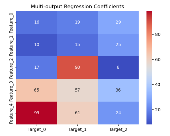

决策树特征重要性

全局特征重要性

# 2. 决策树重要性
from sklearn.tree import DecisionTreeRegressor
from sklearn.inspection import permutation_importance
from sklearn.datasets import make_regression
import pandas as pd
import numpy as np
import matplotlib.pyplot as plt
import seaborn as snsX, y = make_regression(n_targets=3, n_features=5, random_state=42)
# 训练多输出决策树
model = DecisionTreeRegressor(max_depth=3, random_state=42)
model.fit(X, y)# 获取特征重要性
importance = model.feature_importances_
result = permutation_importance(model, X, y, n_repeats=10, random_state=42)# 可视化 - 全局特征重要性
plt.figure(figsize=(10, 4))
pd.Series(importance, index=[f'F_{j}' for j in range(X.shape[1])]) \.plot(kind='bar', title='Global Feature Importance (Averaged across targets)')
plt.tight_layout()
plt.show()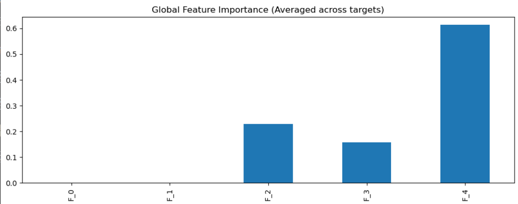

 

每个标签的重要性 

def multi_target_permutation_importance(model, X, y, n_repeats=10, random_state=None):"""计算多目标模型的permutation importance"""results = []for i in range(y.shape[1]):# 创建一个scorer只关注当前目标def scorer(estimator, X, y_true):y_pred = estimator.predict(X)return np.mean((y_pred[:, i] - y_true[:, i]) ** 2)  # MSE for target i# 计算当前目标的permutation importanceresult = permutation_importance(model, X, y, n_repeats=n_repeats,random_state=random_state, scoring=scorer)results.append(result.importances_mean)return np.array(results)# 计算每个目标的permutation importance
target_importances = multi_target_permutation_importance(model, X, y, n_repeats=10, random_state=42)# 转换为DataFrame便于可视化
importance_df = pd.DataFrame(target_importances,columns=[f'F_{j}' for j in range(X.shape[1])],index=[f'Target {i}' for i in range(y.shape[1])])# 可视化 - 每个目标的permutation importance
fig, axes = plt.subplots(1, y.shape[1], figsize=(15, 4))
for i in range(y.shape[1]):importance_df.iloc[i].plot(kind='bar', ax=axes[i], title=f'Target {i} Permutation Importance')
plt.tight_layout()
plt.show()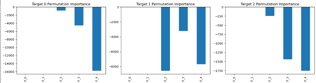

多输出决策树和随机森林解释

# 3. 多输出决策树和随机森林解释
from sklearn.multioutput import MultiOutputRegressor
from sklearn.ensemble import RandomForestRegressor
from sklearn.datasets import make_regression
import numpy as np
import pandas as pd
import matplotlib.pyplot as pltX, y = make_regression(n_targets=3, n_features=5, random_state=42)
# 使用RandomForest作为示例（DecisionTree也可以）
multi_model = MultiOutputRegressor(RandomForestRegressor(max_depth=3, random_state=42))
multi_model.fit(X, y)# 获取每个目标的特征重要性
fig, axes = plt.subplots(1, y.shape[1], figsize=(15, 4))
for i, estimator in enumerate(multi_model.estimators_):pd.Series(estimator.feature_importances_, index=[f'F_{j}' for j in range(X.shape[1])])\.plot(kind='bar', ax=axes[i], title=f'Target {i} Feature Importance')
plt.tight_layout()
plt.show()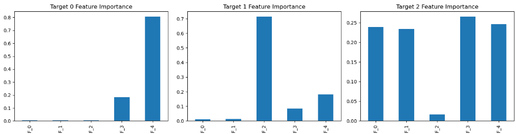

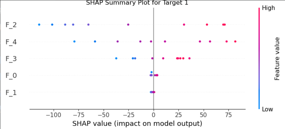
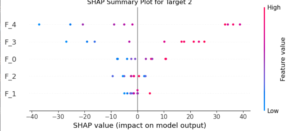
SHAP多目标解释

# 4. SHAP多目标解释
import shap
from sklearn.ensemble import RandomForestRegressor
from sklearn.datasets import make_regression
import numpy as np
import matplotlib.pyplot as pltX, y = make_regression(n_targets=3, n_features=5, random_state=42)
model = RandomForestRegressor(n_estimators=100, random_state=42)
model.fit(X, y)# 创建SHAP解释器
explainer = shap.Explainer(model, X[:100])
shap_values = explainer(X[:10])# 可视化每个目标的SHAP值
for target_idx in range(y.shape[1]):print(f"\nTarget {target_idx} Explanation:")shap.summary_plot(shap_values[:, :, target_idx].values,X[:10],feature_names=[f'F_{i}' for i in range(X.shape[1])],show=False)plt.title(f"SHAP Summary Plot for Target {target_idx}")plt.show()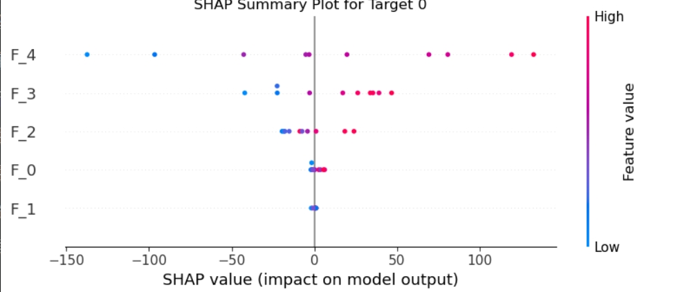

 

 

 

多目标PDP分析

# 5. 多目标PDP分析
from sklearn.inspection import PartialDependenceDisplay
from sklearn.datasets import make_regression
from sklearn.ensemble import RandomForestRegressor
import numpy as np
import matplotlib.pyplot as pltX, y = make_regression(n_targets=3, n_features=5, random_state=42)
model = RandomForestRegressor(n_estimators=100, random_state=42)
model.fit(X, y)fig, axes = plt.subplots(y.shape[1], 3, figsize=(15, 10))
for target_idx in range(y.shape[1]):for feat_idx in [0,1,2]:  # 展示前三个特征PartialDependenceDisplay.from_estimator(model, X, features=[feat_idx],target=target_idx, ax=axes[target_idx, feat_idx])axes[target_idx, feat_idx].set_title(f'Target {target_idx} | Feature {feat_idx}')
plt.tight_layout()
plt.show()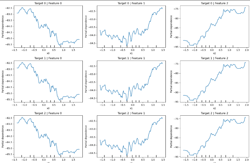

神经注意力解释

# 6. 神经注意力解释
import tensorflow as tf
from tensorflow.keras.layers import MultiHeadAttention, Dense, Input, Reshape
from sklearn.datasets import make_regression
import numpy as np
import seaborn as sns
import matplotlib.pyplot as pltX, y = make_regression(n_targets=3, n_features=5, random_state=42)# 构建带注意力的多输出模型
inputs = Input(shape=(X.shape[1],))
x = Dense(64, activation='relu')(inputs)# 调整形状以适应注意力层 (batch_size, seq_len, embed_dim)
x_reshaped = Reshape((1, 64))(x)  # 添加序列长度为1的维度# 使用MultiHeadAttention
attn_output, attn_weights = MultiHeadAttention(num_heads=4,key_dim=16
)(x_reshaped, x_reshaped, return_attention_scores=True)# 展平注意力输出
attn_flat = tf.keras.layers.Flatten()(attn_output)# 多输出
outputs = [Dense(1, name=f'output_{i}')(attn_flat) for i in range(y.shape[1])]model = tf.keras.Model(inputs=inputs, outputs=outputs)
model.compile(optimizer='adam', loss='mse')# 提取注意力权重
attention_model = tf.keras.Model(inputs=inputs,outputs=model.get_layer('multi_head_attention').output[1]  # 获取注意力权重
)
attn_weights = attention_model.predict(X[:5])
# 调整注意力权重形状为2D (num_heads, seq_len*seq_len)
attn_weights_2d = np.squeeze(attn_weights)  # 从(5,4,1,1)变为(5,4)
attn_weights_2d = attn_weights_2d.T  # 转置为(4,5)# 可视化
plt.figure(figsize=(10,5))
sns.heatmap(attn_weights_2d,annot=True,xticklabels=[f'Sample_{i}' for i in range(5)],yticklabels=[f'Head_{i}' for i in range(4)])
plt.xlabel('Input Samples')
plt.ylabel('Attention Heads')
plt.title('Attention Weights per Head across Samples')
plt.show()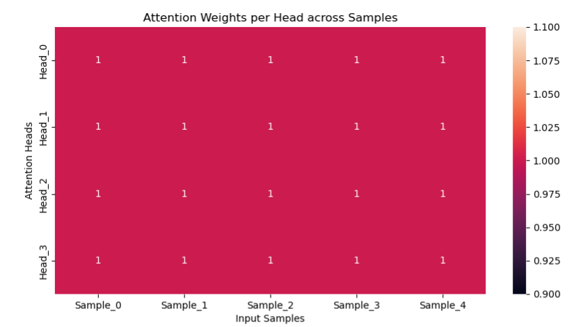

进阶技巧

目标相关性分析

## 进阶技巧
# 1. 目标相关性分析
# 计算目标间相关系数
from sklearn.datasets import make_regression
import numpy as np
import seaborn as sns
import pandas as pd
import matplotlib.pyplot as pltX, y = make_regression(n_targets=3, n_features=5, random_state=42)
target_corr = pd.DataFrame(y).corr()# 可视化目标关系
sns.clustermap(target_corr, annot=True)
plt.title('Inter-target Correlation')
plt.tight_layout()
plt.show()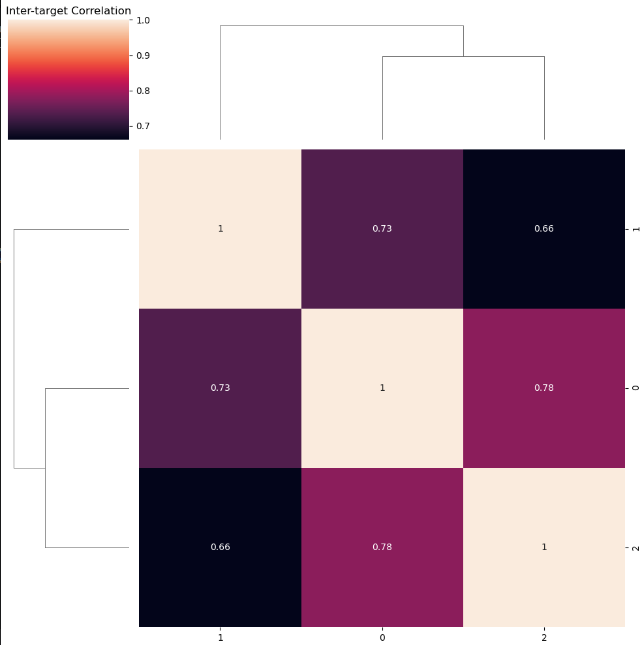

多目标特征交互分析

# 2. 多目标特征交互分析
# 使用SHAP交互值
import shap
import seaborn as sns
from sklearn.datasets import make_regression
from sklearn.ensemble import RandomForestRegressor
import numpy as np
import matplotlib.pyplot as pltX, y = make_regression(n_targets=3, n_features=5, random_state=42)
model = RandomForestRegressor(n_estimators=100, random_state=42)
model.fit(X, y)# 计算SHAP交互值
explainer = shap.TreeExplainer(model)
shap_interaction = explainer.shap_interaction_values(X[:100])  # 形状应为(100,3,5,5)# 计算特征-目标间的平均交互强度
interaction_matrix = np.zeros((y.shape[1], X.shape[1]))
for i in range(y.shape[1]):# 获取当前目标的所有样本的SHAP值 (100,5)target_shap = np.array(shap_interaction)[:,i,:,:].sum(axis=2)  # 沿特征维度求和# 计算平均SHAP值interaction_matrix[i,:] = np.abs(target_shap).mean(axis=0)# 可视化
plt.figure(figsize=(12, 6))
sns.heatmap(interaction_matrix,cmap='viridis',annot=True,fmt=".2f",xticklabels=[f'F_{i}' for i in range(X.shape[1])],yticklabels=[f'T_{i}' for i in range(y.shape[1])])
plt.title('Feature Importance for Each Target')
plt.xlabel('Features')
plt.ylabel('Targets')
plt.tight_layout()
plt.show()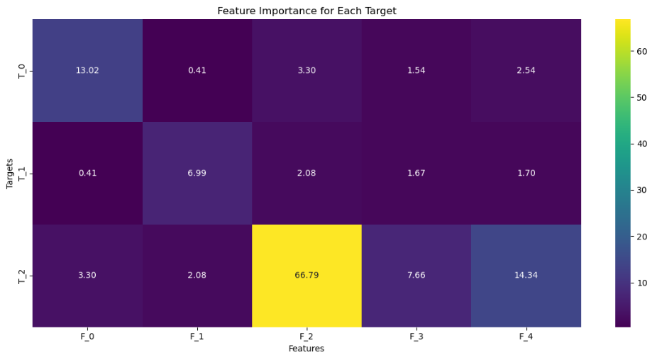

动态解释可视化

# 3. 动态解释可视化
import plotly.express as px
from sklearn.datasets import make_regression
from sklearn.ensemble import RandomForestRegressor
import numpy as np
import matplotlib.pyplot as pltX, y = make_regression(n_targets=3, n_features=5, random_state=42)
model = RandomForestRegressor(n_estimators=100, random_state=42)
model.fit(X, y)# 创建动态PDP图
def interactive_pdp(model, X, feature_idx, target_idx):grid = np.linspace(X[:, feature_idx].min(), X[:, feature_idx].max(), 100)pdp = []for val in grid:X_temp = X.copy()X_temp[:, feature_idx] = valpdp.append(model.predict(X_temp)[:, target_idx].mean())fig = px.line(x=grid, y=pdp,labels={'x': f'Feature {feature_idx}', 'y': 'Prediction'},title=f'Target {target_idx} PDP')fig.show()interactive_pdp(model, X, feature_idx=1, target_idx=0)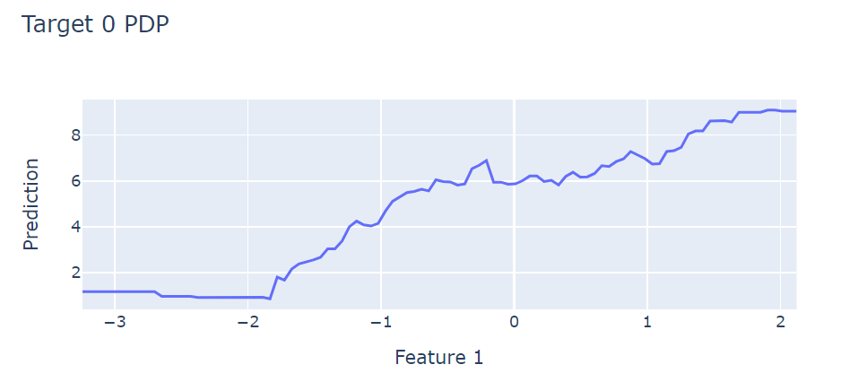

 

方法对比

方法类型	优势	局限性	适用场景
线性模型	全局解释性强	只能捕捉线性关系	特征数<样本数
决策树	非线性关系可视化	容易过拟合	中小规模数据
SHAP分析	统一尺度解释	计算成本高	任何模型
注意力机制	特征交互可视化	需要足够数据	高维特征交互分析
代理模型	可解释黑箱模型	解释是近似的	模型不可解释时