运行时长和内存优化：混合精度训练（MPT）案例和梯度检查点（GCP）

1. 混合精度训练 Mixed Precision Training, MPT

混合精度训练（Mixed Precision Training） 是一种 深度学习优化技术，旨在使用 不同精度的数据类型（如 FP32 和 FP16） 进行训练，以 减少计算开销、降低显存占用，并提高模型训练速度，同时保持与全精度训练相近的模型精度。

这里就直接用一个例子来展示一下MPT的效果

先导入必要的库，其中比较关键的时最后一个GradScalar和autocast

import torch 
import time
import torch.nn as nn
import numpy as np
import matplotlib.pyplot as plt
import seaborn as sns
from torch.cuda.amp import GradScaler, autocastsns.set()

 此书前面的章节介绍了用神经网络构造一个sin-cos多任务训练网络，我们还是以那个栗子来实践，先定义一下数据：

high = 2 * np.pi
x = torch.unsqueeze(torch.linspace(-high, high, 20000), dim=1)
x = x[torch.randperm(x.shape[0])]random_sin = np.random.uniform(low=-0.01, high=0.01, size=(x.shape[0],))
random_cos = np.random.uniform(low=-0.01, high=0.01, size=(x.shape[0],))sin_y = (torch.sin(x[:, 0]) + random_sin).reshape(-1, 1).double()
cos_y = (torch.cos(x[:, 0]) + random_cos).reshape(-1, 1).double()# Move data to GPU if available
device = torch.device("cuda" if torch.cuda.is_available() else "cpu")
x = x.to(device)
sin_y = sin_y.to(device)
cos_y = cos_y.to(device)

 可视化观察一下这个数据的样子

plt.figure(figsize=(6, 4))
plt.scatter(x[:, 0].reshape(-1, 1), sin_y, s=20, label="Sin")
plt.scatter(x[:, 0].reshape(-1, 1), cos_y, s=20, label="Cos")
plt.legend()
plt.show()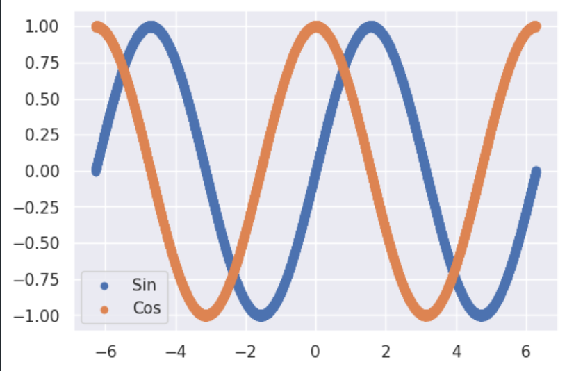

定义一个多任务模型，参数在经过共享网络区域model1后，由model2和model3进行多任务分支训练。 

class Net(nn.Module):def __init__(self, h):super(Net, self).__init__()self.model1 = torch.nn.Sequential(torch.nn.Linear(x.shape[1], h),torch.nn.ReLU(),torch.nn.Linear(h, h),torch.nn.ReLU(),torch.nn.Linear(h, h),torch.nn.ReLU()  )self.model_sin = torch.nn.Sequential(torch.nn.Linear(h, h),torch.nn.ReLU(),torch.nn.Linear(h, 1))self.model_cos = torch.nn.Sequential(torch.nn.Linear(h, h),torch.nn.ReLU(),torch.nn.Linear(h, 1))def forward(self, inputs):x1 = self.model1(inputs)output_sin = self.model_sin(x1).double()output_cos = self.model_cos(x1).double()return output_sin, output_cos

为了便于观察， 我们分别定义两个训练函数，分别是使用MTP和不适用MTP：

def train_without_mixed_precision(epochs=100, learning_rate=0.01):"""训练函数 - 不使用混合精度"""net = Net(150).to(device)losses = []loss_func = torch.nn.MSELoss()optimizer = torch.optim.Adam(net.parameters(), lr=learning_rate)start_time = time.time()for epoch in range(epochs):optimizer.zero_grad()prediction = net(x)loss1 = loss_func(prediction[0], sin_y)loss2 = loss_func(prediction[1], cos_y)loss = loss1 + loss2loss.backward()optimizer.step()losses.append(loss.item())if (epoch + 1) % 20 == 0:print(f"Regular Training - Epoch = {epoch}, Loss = {round(loss.item(), 3)}")end_time = time.time()training_time = end_time - start_timereturn losses, training_timedef train_with_mixed_precision(epochs=100, learning_rate=0.01):"""训练函数 - 使用混合精度"""net = Net(150).to(device)losses = []loss_func = torch.nn.MSELoss()optimizer = torch.optim.Adam(net.parameters(), lr=learning_rate)scaler = GradScaler(enabled=True)start_time = time.time()for epoch in range(epochs):optimizer.zero_grad()with autocast():prediction = net(x)loss1 = loss_func(prediction[0], sin_y)loss2 = loss_func(prediction[1], cos_y)loss = loss1 + loss2scaler.scale(loss).backward()scaler.step(optimizer)scaler.update()losses.append(loss.item())if (epoch + 1) % 20 == 0:print(f"Mixed Precision Training - Epoch = {epoch}, Loss = {round(loss.item(), 3)}")end_time = time.time()training_time = end_time - start_timereturn losses, training_time

 接下俩就运行他，加一些结果记录的输出信息：

# 运行对比实验
epochs = 1000
learning_rate = 0.01print("=== 开始训练对比实验 ===")
print(f"Device: {device}")
print(f"Epochs: {epochs}")
print(f"Learning Rate: {learning_rate}")
print(f"Data Size: {x.shape[0]}")
print()# 不使用混合精度训练
print("1. 开始常规训练（不使用混合精度）...")
regular_losses, regular_time = train_without_mixed_precision(epochs, learning_rate)
print(f"常规训练完成，耗时: {regular_time:.2f} 秒")
print()# 使用混合精度训练
print("2. 开始混合精度训练...")
mixed_losses, mixed_time = train_with_mixed_precision(epochs, learning_rate)
print(f"混合精度训练完成，耗时: {mixed_time:.2f} 秒")
print()# 计算加速比和时间节省
speedup = regular_time / mixed_time
time_saved = regular_time - mixed_time
time_saved_percent = (time_saved / regular_time) * 100print("=== 训练对比结果 ===")
print(f"常规训练时间: {regular_time:.2f} 秒")
print(f"混合精度训练时间: {mixed_time:.2f} 秒")
print(f"时间节省: {time_saved:.2f} 秒 ({time_saved_percent:.1f}%)")
print(f"加速比: {speedup:.2f}x")

 你应该能看到类似的结果：

常规训练时间: 3.11 秒
混合精度训练时间: 2.13 秒
时间节省: 0.99 秒 (31.6%)
加速比: 1.46x

 下面是一些可视化的对比图，需要的话可以私我（或者让gpt帮忙一下~~~）

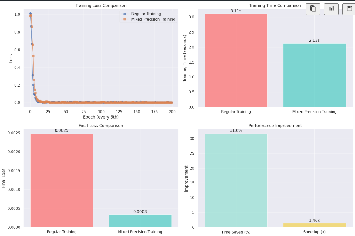
 需要注意的是，对于简单模型+小轮次训练，MTP的效果并不突出，也是，其本来就是缓解大规模训练导致的耗时问题的，在尝试代码的时候可以将epoch调大一点哈哈哈试一下。

2. 梯度检查点 Gradient Checkpointing, GCP

神经网络主要通过两种方式占用内存：

(1). 权重参数——————————静态占用

(2). 向前或向后传播时的计算———动态占用

而模型内存的占用和batch size的尺寸几乎正比关系，因此，如果能保持整体内存利用率的同时增大batch，那是自然好的，梯度检查点就是用来干这个。

2.1 GCP工作过程

GCP主要依赖两个神经网络训练过程中涉及到的先验知识：

前提1：某一层的激活值，仅依赖前一层的激活值

举个栗子，对于LayerB的激活，其等于

其中是LayerB的权重，是偏执项，是激活函数，如ReLU，Sigmod等。Layer B 的激活 只需要前一层（Layer A）的激活值，以及自身的权重 / 偏置，和前层无关。 

前提2：更新某一层的权重只依赖（1）该层自身的激活值（前向传播的结果）；（2）下一层（右侧层）计算出的梯度（反向传播的结果）

基于这两个前提，GCP就可以工作了。

Step1：向前传播前，将网络划分成两个分段（Segement）

Step2：在向前传播过程中，只存储每个分段中第一层的激活。其余部分被用于计算下一层的激活后丢弃。

Step3：向后传播时，当某一层需要更新权重的时候，需要用到自身的激活，问题来了，自身激活在Step2中丢弃了，怎么办？

我们还保留了该分段中的第一层的激活，重新计算当前层激活就好。如此一来，在训练过程中无需保存中间层众多的参数，在反向传播中重新计算便可。

不难发现，这是一种典型的时间换空间的方案，因为一些激活值被计算了两次，计算时间会增加15%-25%，但内容占用却能大幅降低（作者所示的数据中能够降低50%-60%），

2.2 Pytorch实现

import torch
import torch.nn as nn
from torch.utils.checkpoint import checkpoint_sequentialclass SimpleNet(nn.Module):def __init__(self):super(SimpleNet, self).__init__()self.layer1 = nn.Linear(10, 20)self.layer2 = nn.Linear(20, 30)self.layer3 = nn.Linear(30, 40)def  forward(self, x1):layers = torch.nn.Sequential(self.layer1,nn.ReLU(),self.layer2,nn.ReLU(),self.layer3)# 下面这行最关键x = checkpoint_sequential(layers, segments=2, input=x1)return x