大模型推理 memory bandwidth bound (5) - Medusa

系列文章目录

大模型推理 & memory bandwidth bound (1) - 性能瓶颈与优化概述
大模型推理 & memory bandwidth bound (2) - Multi-Query Attention
大模型推理 & memory bandwidth bound (3) - MLA
大模型推理 & memory bandwidth bound (4) - Speculative Decoding
大模型推理 & memory bandwidth bound (5) - Medusa

---

---

前言

“The inefficiency of Large Language Model (LLM) inference is primarily attributed to the memory-bandwidth-bound nature of the auto-regressive decoding process.” —— 《MEDUSA: Simple LLM Inference Acceleration Framework with Multiple Decoding Heads》

上一篇我们对工作《Fast Inference from Transformers via Speculative Decoding》进行了讲解，对大模型推理加速范式Speculative Decoding有了基本的认识。尽管上述工作设计简洁，但在实际场景中有如下问题需要克服：1）需要额外训练一个draft model，且尽可能保持其输出分布与target model一致；2）将draft model一同集成到分布式系统中具有挑战性。
对于1）补充说明一下：尽管开源模型系列通常包含不同尺寸的模型，且它们的分布相近，但这并不意味着其中必然存在一个合适的小模型作为draft model。以LLaMA2为例，模型尺寸有7B、13B 和 70B。当target model为7B模型时，没有更小的模型作为draft model；而当target model为13B模型时，选择7B模型作为draft model也是不合适的。
为应对上述困难，Medusa应运而生。它承袭了Blockwise Parallel Decoding使用多个解码头的思想，配合tree attention，实现了 >2X 的推理加速，是基于self-drafting的经典工作之一。简单来说，Medusa在target model上加了若干个解码头，取代draft model，并行预测后续若干个token，一个模型打两份工：draft和verify。

---

一、原理

根据论文的介绍，Medusa的重要组成部分是Medusa heads、Tree attention以及Typical acceptance。Medusa heads是用来实现draft model的功能的，而后两者则是在提升acceptance rate上做文章。接下来我们快速过一下，目标是对Medusa原理有一个感性的认识。

1.Medusa heads

和Blockwise Parallel Decoding的做法类似，为了能够并行预测后续多个token，Medusa在模型最后一层追加了若干个解码头，这些解码头区别于模型原始的解码头LM head，被称作Medusa heads。如下图所示，Medusa heads个数为3，加上LM head，实际上并行预测了4个token，只不过后3个token需要做verify。另外，图中显示Medusa在做top-k采样，这一点区别于Blockwise Parallel Decoding，Blockwise Parallel Decoding仅限于Greedy search。

Medusa head的设计比较简单，就是一个残差块，如下面公式所示，其中 $t$ 是当前位置，$k$ 表示第 $k$ 个Medusa head。
$$\begin{array}{r}{p}_t^{(k)}=\text{softmax}(W_2^{(k)}\cdot (\text{SiLU}(W_1^{(k)}\cdot h_t)+h_t)),\\ \text{where}{W}_2^{(k)}\in {\mathbb{R}}^{d\times V},W_1^{(k)}\in {\mathbb{R}}^{d\times d}\end{array}$$

2.Tree attention

根据作者在博客中的描述，相较于使用top-1预测，top-5预测的准确率得到大幅提升，意味着acceptance rate的提升，以及进一步的推理加速。多个解码头的top-k预测做笛卡尔积，组合得到了多个候选生成路径。由于路径比较多，如果我们以batch方式去处理的话是不划算的。比较高效的处理方式是维护一棵树，并从这棵树中找到最优路径。相应的，我们还需要对causal attention做一点改动以适应这种树状数据结构，就有了Tree attention。
下图是使用Tree attention处理多个候选的示意图。图中Root表示模型原始解码头LM head，Medusa head 1做top-2预测，Medusa head 2做top-3预测，那么得到的候选路径有6条。Tree attention把树状结构平铺到一个序列中，调整attention mask使得当前节点只能access到它的predecessors，简单来说就是不被其他路径上的token干扰。举例说明如下：第6行，对应的候选路径是[“I”, “is”]，当前节点（Query）是"is"，它的Key只有自己，以及父节点"I"，对应图中2列和第6列的勾。

然而，作者并没有直接使用这种原始的稠密的树，而是对树进行了稀疏化处理，其背后的原因还是加速效果和计算量的权衡。假设每个Medusa head都按照top-10采样，那么4个Medusa head将会导致树上有1+10+100+1000+10000个candidate tokens（其中1代表根节点），这是一棵庞大的树。而这里面有很多路径概率是很低的，可以被优化掉。下图就是稀疏化之后的树，同样也是top-10采样，总共只有64个节点（candidate tokens），42条路径（比如红色箭头所示的就是其中一条），相比之下这棵树就小得多。需要注意的是，在Medusa中，这棵稀疏化的树是事先构建好的，而不是在推理过程中动态构建的。

下图是acceleration rate以及speed关于candidate tokens数量的变化趋势图，其中蓝色点对应的是稠密树，而红星对应的是稀疏化的树。图中显示了以下几点：1）稀疏化的树推理加速效果显然更好；2）尽管随着candidate tokens数量的增加，acceleration rate也在增加，但是speed只在candidate tokens数量超过80之后在持续下降；acceleration rate表达的是接受长度，当candidate tokens增加，找到一条更长的被接受的路径是必然的，而speed是实际的加速效果，它下降是因为模型处理candidate tokens较多，已经处于compute-bound状态，耗时增加。

3.Typical acceptance

在处理Medusa的采样时，作者采用了Typical acceptance方案，具体表现为如下公式：
$$\begin{array}{r}{p}_{\text{original}}(x_{n+k}|x_1,x_2,\cdot \cdot \cdot ,x_{n+k-1})>\\ \min (ϵ,\delta \exp (-H(p_{\text{original}}(\cdot |x_1,x_2,\cdot \cdot \cdot ,x_{n+k-1}))))\end{array}$$
其中 $ϵ$ 和 $\delta$ 是参数，$H(\cdot )$ 为熵。简单理解这个公式就是target model在候选token $x_{n+k}$ 上的概率超过不等式右侧的阈值才能被接受。从直觉上来讲，这是合理的，因为采样通常会选择概率较高的token。为了深入理解Typical acceptance的内涵，我们需要简单过一遍typical sampling和η-sampling。

【typical sampling】
作者从信息论出发，依据信息量和条件熵的接近程度构造token的候选集，用公式表示如下：
$$L_{ϵ}^{(T)}=\mathbf{y}=y_0\cdot \cdot \cdot y_T|\forall 1\le t\le T,|\log p(y_t|{\mathbf{y}}_{<\mathbf{t}})+H(Y_t|{\mathbf{Y}}_{<\mathbf{t}}={\mathbf{y}}_{<\mathbf{t}})|<ϵ$$
其中 $ϵ$ 是参数， $-\log p(y_t|{\mathbf{y}}_{<\mathbf{t}})$ 是信息量， $H(Y_t|{\mathbf{Y}}_{<\mathbf{t}}={\mathbf{y}}_{<\mathbf{t}})$ 是条件熵，具体表达式为
$$H(Y_t|{\mathbf{Y}}_{<\mathbf{t}}={\mathbf{y}}_{<\mathbf{t}})=-\sum p(y_t|{\mathbf{y}}_{<\mathbf{t}})\cdot \log p(y_t|{\mathbf{y}}_{<\mathbf{t}})$$
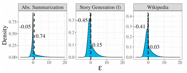
typical sampling使得模型输出既不让人感到惊讶（低概率），也不过分确定（极高概率）。作者给出了一些语料分析以支持typical sampling，下图给出了在不同语料中 $ϵ$ 的分布情况，其中点线指示中位数，虚线指示平均数。因此，通过typical sampling能够生成更加自然，且符合人类语言使用习惯的文本。

(https://arxiv.org/abs/2202.00666)

【η-sampling】
η-sampling在《Truncation Sampling as Language Model Desmoothing》中提出，可认为是对typical sampling的改进，用公式表示如下：
A x < i = { x ∈ V ∣ P θ ( x ∣ x < i ) > η } , η = min ⁡ ( ϵ , α exp ⁡ ( − h θ , x < i ) ) A_{x_{<i}}=\{x \in V|P_\theta(x|x_{<i}) > \eta \},\\ \eta=\min(\epsilon,\alpha \exp(-h_{\theta,x_{<i}})) Ax<i​​={x∈V∣Pθ​(x∣x<i​)>η},η=min(ϵ,αexp(−hθ,x<i​​))
其中 $A_{x_{<i}}$ 是allow set，也就是token候选集， $V$ 是词表，阈值 $\eta$ 由固定参数 $ϵ$ 以及条件熵相关项 $\alpha \exp (-h_{\theta ,x_{<i}})$ 共同决定。

1）不考虑 $ϵ$ 项，并对上式两边取对数，会发现和typical sampling形式非常类似，只是相比之下typical sampling对token候选集的要求更严苛，因为其表达式中的绝对值符号表明它筛选token时同时设置了概率上限和下限，而η-sampling只设置了概率下限，允许概率更大的token被采样；
2） $ϵ$ 项是对1）的补充，直观理解是候选集中token的概率不至于过低。

到此我们实际上已经把Typical acceptance说清楚了，因为你发现其表达式和η-sampling是一致的。

【truncation sampling的新视角】
η-sampling是在论文《Truncation Sampling as Language Model Desmoothing》中提出的。顺带提一下，该论文提供了一个全新的视角来理解LLM采样前的 truncation 过程（只在概率较大的token中采样，比如top-k、top-p）。如下图所示，作者认为LLM中的概率分布是真实分布和平滑分布的叠加，truncation 的目标是去平滑以近似真实分布。

(https://arxiv.org/abs/2210.15191)

【typical acceptance】
现在来解释为什么在Medusa中采用typical acceptance这种采样方法。1）作者认为，在真实场景中采样是用于生成不同的回答的，像Speculative Sampling那样使得输出分布与原始模型分布严格对齐的做法不是必需的，只要选择plausible的token即可；2）上一篇我们已经提到，Speculative Sampling会导致推理加速效率随着采样温度的升高而降低；使用typical acceptance则没有这个问题，随着温度的升高，被接受的序列长度反而增加了，也即获得更大的加速比。

4.Train

针对不同的使用场景，提供了两种不同的微调流程：
MEDUSA-1：资源受限，固定backbone，只训练Medusa heads；
MEDUSA-2：计算资源充足，backbone和Medusa heads联合训练，能获得更大的加速比。
MEDUSA-1的loss如下，对数部分表示第 $k$ 个Medusa head预测 $t+k+1$ 位置的token时的交叉熵损失， ${\lambda }_k$ 成指数衰减，比如 $0.8^k$ 。
$$L_{\text{MEDUSA-1}}=\sum _{k=1}^K-{\lambda }_k\log p_t^{(k)}(y_{t+k+1})$$
MEDUSA-2需要将LM head考虑在内，其loss形式如下：
$$L_{\text{MEDUSA-2}}=L_{LM}+{\lambda }_0{L}_{\text{MEDUSA-1}}$$
论文中还给了一些训练的tricks，这里就不赘述了。

二、代码

这边提一句，在medusa_model.py中默认设置medusa_num_heads=5，huggingface上的模型medusa-vicuna-7b-v1.3也是训练了5个Medusa heads，但是medusa_choices.py中的树结构实际对应的Medusa_heads个数是4，所以我们理论上应修改配置为medusa_num_heads=4。

1.medusa_generate()

Medusa生成依赖于medusa_generate()方法，步骤概括如下（这里刚开始不懂没关系，后面会对每个方法单独讲解）：
1）self.get_medusa_choice()获取稀疏树结构；
2）generate_medusa_buffers()对树结构做数据处理，得到更容易被消费的数据；
3）initialize_medusa()对输入做prefill，并得到logits和medusa_logits；
4）generate_candidates()生成candidate tokens，并将树上的candidate tokens平铺到一个序列中；
5）tree_decoding()对4）中序列做解码；
6）evaluate_posterior()通过typical acceptance做Verify，选择最优路径；
7）update_inference_inputs()更新得到新序列，准备下一轮。

    def medusa_generate(self,input_ids,attention_mask=None,temperature=0.0,max_steps=512,# The hyperparameters below are for the Medusa# top-1 prediciton for the next token, top-7 predictions for the next token, top-6 predictions for the next next token.medusa_choices=None,posterior_threshold=0.09,  # threshold validation of Medusa output# another threshold hyperparameter, recommended to be sqrt(posterior_threshold)posterior_alpha=0.3,top_p=0.8, sampling = 'typical', fast = True):"""Args:input_ids (torch.Tensor, optional): Input token IDs.attention_mask (torch.Tensor, optional): Attention mask.temperature (float, optional): Temperature for typical acceptance.medusa_choices (list, optional): A list of integers indicating the number of choices for each Medusa head.posterior_threshold (float, optional): Threshold for posterior validation.posterior_alpha (float, optional): Another threshold hyperparameter, recommended to be sqrt(posterior_threshold).top_p (float, optional): Cumulative probability threshold for nucleus sampling. Defaults to 0.8.sampling (str, optional): Defines the sampling strategy ('typical' or 'nucleus'). Defaults to 'typical'.fast (bool, optional): If True, enables faster, deterministic decoding for typical sampling. Defaults to False.Returns:torch.Tensor: Output token IDs.Warning: Only support batch size 1 for now!!"""# ...# 获取medusa_choices，也就是稀疏树结构medusa_choices = self.get_medusa_choice(self.base_model_name_or_path)# 获取树数据做处理，方便后面消费# Initialize the medusa buffermedusa_buffers = generate_medusa_buffers(medusa_choices, device=self.base_model.device)self.medusa_buffers = medusa_buffersself.medusa_choices = medusa_choices# ...# 初始化并作prefill，foward拿到medusa_logits, logits# Initialize tree attention mask and process prefill tokensmedusa_logits, logits = initialize_medusa(input_ids, self, medusa_buffers["medusa_attn_mask"], past_key_values)new_token = 0last_round_token = 0for idx in range(max_steps):# 生成candidate_tokens，并将树结构平铺到一个序列中# Generate candidates with topk predictions from Medusa headscandidates, tree_candidates = generate_candidates(medusa_logits,logits,medusa_buffers["tree_indices"],medusa_buffers["retrieve_indices"],temperature=temperature,posterior_alpha=posterior_alpha,posterior_threshold=posterior_threshold,top_p=top_p,sampling=sampling,fast=fast,)# 对平铺的序列做解码# Use tree attention to verify the candidates and get predictionsmedusa_logits, logits, outputs = tree_decoding(self,tree_candidates,past_key_values,medusa_buffers["medusa_position_ids"],input_ids,medusa_buffers["retrieve_indices"],)# 通过typical acceptance做Verify，选择最优路径# Evaluate the posterior of the candidates to select the accepted candidate prefixbest_candidate, accept_length = evaluate_posterior(logits, candidates, temperature, posterior_threshold, posterior_alpha, top_p=top_p, sampling=sampling, fast=fast)# 将树结构移除，把最优路径append到input上得到新的input# Update the input_ids and logitsinput_ids, logits, medusa_logits, new_token = update_inference_inputs(input_ids,candidates,best_candidate,accept_length,medusa_buffers["retrieve_indices"],outputs,logits,medusa_logits,new_token,past_key_values_data,current_length_data,)yield {"text": self.tokenizer.decode(input_ids[0, input_len:],skip_special_tokens=True,spaces_between_special_tokens=False,clean_up_tokenization_spaces=True,)}if self.tokenizer.eos_token_id in input_ids[0, input_len:]:break

2.generate_medusa_buffers()

def generate_medusa_buffers(medusa_choices, device="cuda"):"""Generate buffers for the Medusa structure based on the provided choices.Parameters:- device (str): Device to which the tensors should be moved. Default is "cuda".Returns:- dict: A dictionary containing buffers related to the Medusa structure."""# ... 解析tree的代码逻辑不重要，见下面举例说明# 返回以下几项数据# Aggregate the generated buffers into a dictionarymedusa_buffers = {"medusa_attn_mask": medusa_attn_mask.unsqueeze(0).unsqueeze(0),"tree_indices": medusa_tree_indices,"medusa_position_ids": medusa_position_ids,"retrieve_indices": retrieve_indices,}# Move the tensors in the dictionary to the specified devicemedusa_buffers = {k: v.clone().to(device)if isinstance(v, torch.Tensor)else torch.tensor(v,  device=device)for k, v in medusa_buffers.items()}return medusa_buffers

方法generate_medusa_buffers()的作用是对已知的树结构做解析，以便后续模型处理。由于这只是基于逻辑的处理，具体代码逐行分析没有实际举例来的直观，我将结合下图对该方法进行说明。

先来回顾下这棵树，这棵树的根节点是LM head预测的token，下面四层是4个Medusa heads预测的token。LM head使用的是greedy search，只有一个token，而Medusa heads全部使用top-10采样，当然这边稀疏化处理砍掉了一些节点。这棵树共有64个节点（蓝色点），42条路径（如红色路径）。
现在开始对generate_medusa_buffers()的输入输出举例说明。输入：

• medusa_choices：树的节点表达，不包括根节点，比如上图中的红色路径节点 ‘upon’ 用 (0,) 表示， ‘a’ 用 (0, 1) 表示，‘time’ 用 (0, 1, 0) 表示，这种表达方式记录了从根节点到该节点的路径。

# medusa_choices，元素个数为63
[(0,), (0, 0), (1,), (0, 1), (0, 0, 0), (1, 0), (2,), (0, 2), (0, 0, 1), (0, 3), (3,), (0, 1, 0), (2, 0), (4,), (0, 0, 2), (0, 4), (1, 1), (1, 0, 0), (0, 0, 0, 0), (5,), (0, 0, 3), (0, 5), (0, 2, 0), (3, 0), (0, 1, 1), (0, 6), (6,), (0, 7), (0, 0, 4), (4, 0), (1, 2), (0, 8), (7,), (0, 3, 0), (0, 0, 0, 1), (0, 0, 5), (2, 1), (0, 0, 6), (1, 0, 1), (0, 0, 1, 0), (2, 0, 0), (5, 0), (0, 9), (0, 1, 2), (8,), (0, 4, 0), (0, 2, 1), (1, 3), (0, 0, 7), (0, 0, 0, 2), (0, 0, 8), (1, 1, 0), (0, 1, 0, 0), (6, 0), (9,), (0, 1, 3), (0, 0, 0, 3), (1, 0, 2), (0, 5, 0), (3, 1), (0, 0, 2, 0), (7, 0), (1, 4)]# sorted_medusa_choices
[(0,), (1,), (2,), (3,), (4,), (5,), (6,), (7,), (8,), (9,), (0, 0), (0, 1), (0, 2), (0, 3), (0, 4), (0, 5), (0, 6), (0, 7), (0, 8), (0, 9), (1, 0), (1, 1), (1, 2), (1, 3), (1, 4), (2, 0), (2, 1), (3, 0), (3, 1), (4, 0), (5, 0), (6, 0), (7, 0), (0, 0, 0), (0, 0, 1), (0, 0, 2), (0, 0, 3), (0, 0, 4), (0, 0, 5), (0, 0, 6), (0, 0, 7), (0, 0, 8), (0, 1, 0), (0, 1, 1), (0, 1, 2), (0, 1, 3), (0, 2, 0), (0, 2, 1), (0, 3, 0), (0, 4, 0), (0, 5, 0), (1, 0, 0), (1, 0, 1), (1, 0, 2), (1, 1, 0), (2, 0, 0), (0, 0, 0, 0), (0, 0, 0, 1), (0, 0, 0, 2), (0, 0, 0, 3), (0, 0, 1, 0), (0, 0, 2, 0), (0, 1, 0, 0)]

输出：

• medusa_attn_mask：shape为(medusa_len, medusa_len)，其中medusa_len=64为树上所有节点的个数，包括根节点；参照原理部分Tree attention图中的Tree mask，在打勾的位置设置mask值为1；由于包含了根节点，第一列都为1；

# medusa_attn_mask, shape: (medusa_len, medusa_len)
tensor([[1., 0., 0.,  ..., 0., 0., 0.],[1., 1., 0.,  ..., 0., 0., 0.],[1., 0., 1.,  ..., 0., 0., 0.],...,[1., 1., 0.,  ..., 1., 0., 0.],[1., 1., 0.,  ..., 0., 1., 0.],[1., 1., 0.,  ..., 0., 0., 1.]])

• tree_indices：当前节点对应的token在所有token中的索引，就以红色路径最优一个节点对应的token ‘,’ 为例，LM head采样token个数为1，前3个Medusa head各采样10个token，总共为31个token，token ‘,’ 为第4个Medusa head采样的第一个token，总的来看就是第32个token，因此它在所有token中的索引是31；

# tree_indices, shape: (medusa_len, medusa_len)
tensor([ 0,  1,  2,  3,  4,  5,  6,  7,  8,  9, 10, 11, 12, 13, 14, 15, 16, 17,18, 19, 20, 11, 12, 13, 14, 15, 11, 12, 11, 12, 11, 11, 11, 11, 21, 22,23, 24, 25, 26, 27, 28, 29, 21, 22, 23, 24, 21, 22, 21, 21, 21, 21, 22,23, 21, 21, 31, 32, 33, 34, 31, 31, 31])

• medusa_position_ids：这个很好理解，就是每个节点所在层数，比如根节点就在第0层；

# medusa_position_ids, shape: (medusa_len, )
tensor([0, 1, 1, 1, 1, 1, 1, 1, 1, 1, 1, 2, 2, 2, 2, 2, 2, 2, 2, 2, 2, 2, 2, 2,2, 2, 2, 2, 2, 2, 2, 2, 2, 2, 3, 3, 3, 3, 3, 3, 3, 3, 3, 3, 3, 3, 3, 3,3, 3, 3, 3, 3, 3, 3, 3, 3, 4, 4, 4, 4, 4, 4, 4])

• retrieve_indices：42条路径，每条路径上每个节点在64个节点中的索引，节点缺失的部分用-1填充。

# retrieve_indices, shape: (5, 42)
tensor([[ 0,  1, 12, 43, 63],[ 0,  1, 11, 36, 62],[ 0,  1, 11, 35, 61],[ 0,  1, 11, 34, 60],[ 0,  1, 11, 34, 59],[ 0,  1, 11, 34, 58],[ 0,  1, 11, 34, 57],[ 0,  3, 26, 56, -1],[ 0,  2, 22, 55, -1],[ 0,  2, 21, 54, -1],[ 0,  2, 21, 53, -1],[ 0,  2, 21, 52, -1],[ 0,  1, 16, 51, -1],[ 0,  1, 15, 50, -1],[ 0,  1, 14, 49, -1],[ 0,  1, 13, 48, -1],[ 0,  1, 13, 47, -1],[ 0,  1, 12, 46, -1],[ 0,  1, 12, 45, -1],[ 0,  1, 12, 44, -1],[ 0,  1, 11, 42, -1],[ 0,  1, 11, 41, -1],[ 0,  1, 11, 40, -1],[ 0,  1, 11, 39, -1],[ 0,  1, 11, 38, -1],[ 0,  1, 11, 37, -1],[ 0,  8, 33, -1, -1],[ 0,  7, 32, -1, -1],[ 0,  6, 31, -1, -1],[ 0,  5, 30, -1, -1],[ 0,  4, 29, -1, -1],[ 0,  4, 28, -1, -1],[ 0,  3, 27, -1, -1],[ 0,  2, 25, -1, -1],[ 0,  2, 24, -1, -1],[ 0,  2, 23, -1, -1],[ 0,  1, 20, -1, -1],[ 0,  1, 19, -1, -1],[ 0,  1, 18, -1, -1],[ 0,  1, 17, -1, -1],[ 0, 10, -1, -1, -1],[ 0,  9, -1, -1, -1]])

所以该方法只是在做数据处理，仅此而已。

3.initialize_medusa()

def initialize_medusa(input_ids, model, medusa_attn_mask, past_key_values):"""Initializes the Medusa structure for a given model.This function performs the following operations:1. Forward pass through the model to obtain the Medusa logits, original model outputs, and logits.2. Sets the Medusa attention mask within the base model.Args:- input_ids (torch.Tensor): The input tensor containing token ids.- model (MedusaLMHead): The model containing the Medusa layers and base model.- medusa_attn_mask (torch.Tensor): The attention mask designed specifically for the Medusa structure.- past_key_values (list of torch.Tensor): Contains past hidden states and past attention values.Returns:- medusa_logits (torch.Tensor): Logits from the Medusa heads.- logits (torch.Tensor): Original logits from the base model."""medusa_logits, outputs, logits = model(input_ids, past_key_values=past_key_values, output_orig=True, medusa_forward=True)model.base_model.model.medusa_mask = medusa_attn_mask  # 之前清空，这里赋值return medusa_logits, logits

该方法的作用是初始化tree attention mask，并且做prefill。其输入medusa_attn_mask之前已经讲过，也就是64节点的树结构平铺成一个序列后做的mask。输出为medusa_logits和logits，medusa_logits是Medusa heads的输出，形状为(num_medusa_head, 1, seq_len, vocab_size)，logits是LM head的输出，形状为(1, seq_len, vocab_size)。

4.generate_candidates()

该方法根据前面得到的medusa_logits，logits，tree_indices以及retrieve_indices生成candidate tokens，最终输出cart_candidates和tree_candidates。cart_candidates形状与retrieve_indices相同，为(42, 5)，是做笛卡尔积获得42条路径的结果；tree_candidates形状为(1, medusa_len)，是64个节点对应的token。具体实现步骤已在代码中注释。

def generate_candidates(medusa_logits, logits, tree_indices, retrieve_indices, temperature = 0, posterior_threshold=0.3, posterior_alpha = 0.09, top_p=0.8, sampling = 'typical', fast = False):"""Generate candidates based on provided logits and indices.Parameters:- medusa_logits (torch.Tensor): Logits from a specialized Medusa structure, aiding in candidate selection.- logits (torch.Tensor): Standard logits from a language model.- tree_indices (list or torch.Tensor): Indices representing a tree structure, used for mapping candidates.- retrieve_indices (list or torch.Tensor): Indices for extracting specific candidate tokens.- temperature (float, optional): Controls the diversity of the sampling process. Defaults to 0.- posterior_threshold (float, optional): Threshold for typical sampling. Defaults to 0.3.- posterior_alpha (float, optional): Scaling factor for the entropy-based threshold in typical sampling. Defaults to 0.09.- top_p (float, optional): Cumulative probability threshold for nucleus sampling. Defaults to 0.8.- sampling (str, optional): Defines the sampling strategy ('typical' or 'nucleus'). Defaults to 'typical'.- fast (bool, optional): If True, enables faster, deterministic decoding for typical sampling. Defaults to False.Returns:- tuple (torch.Tensor, torch.Tensor): A tuple containing two sets of candidates:1. Cartesian candidates derived from the combined original and Medusa logits.2. Tree candidates mapped from the Cartesian candidates using tree indices."""# Greedy decoding: Select the most probable candidate from the original logits.if temperature == 0 or fast:# 走这个分支---> fast = True，按照论文所说根节点走greedy search，candidates_logit：(1,)candidates_logit = torch.argmax(logits[:, -1]).unsqueeze(0)else:if sampling == 'typical':candidates_logit = get_typical_one_token(logits[:, -1], temperature, posterior_threshold, posterior_alpha).squeeze(0)elif sampling == 'nucleus':candidates_logit = get_nucleus_one_token(logits[:, -1], temperature, top_p).squeeze(0)else:raise NotImplementedError# medusa_logits:(num_medusa_head, 1, seq_len, vocab_size) -> candidates_medusa_logits: (num_medusa_head, topk)，实际是indices而不是logits# Extract the TOPK candidates from the medusa logits.candidates_medusa_logits = torch.topk(medusa_logits[:, 0, -1], TOPK, dim = -1).indices# candidates: (41, ), 10+1个token# Combine the selected candidate from the original logits with the topk medusa logits.candidates = torch.cat([candidates_logit, candidates_medusa_logits.view(-1)], dim=-1)# tree_candidates: (64, ), 每个节点对应的token# Map the combined candidates to the tree indices to get tree candidates.tree_candidates = candidates[tree_indices]# 最后补一个0，应对路径中用-1表示的节点# Extend the tree candidates by appending a zero.tree_candidates_ext = torch.cat([tree_candidates, torch.zeros((1), dtype=torch.long, device=tree_candidates.device)], dim=0)  # torch.Size([65])# cart_candidates: 和retrieve_indices形状相同，(路径个数, 层数)，也就是 (42, 5)# Retrieve the cartesian candidates using the retrieve indices.cart_candidates = tree_candidates_ext[retrieve_indices]# Unsqueeze the tree candidates for dimension consistency.tree_candidates = tree_candidates.unsqueeze(0)return cart_candidates, tree_candidates

5.tree_decoding()

上述generate_candidates()将树结构平铺得到tree_candidates，而tree_decoding()将对这部分做解码。换句话说，每个节点上的token都过一遍LM head和4个Medusa head，计算medusa_logits和logits。这一步的作用是什么呢？
1）logits的计算是为了后面做Verify；
2）而medusa_logits是为了将下一轮的Draft与当前轮的Verify放到一起做，而不用分开让模型forward两次，效率更高。

def tree_decoding(model,tree_candidates,past_key_values,medusa_position_ids,input_ids,retrieve_indices,
):"""Decode the tree candidates using the provided model and reorganize the logits.Parameters:- model (nn.Module): Model to be used for decoding the tree candidates.- tree_candidates (torch.Tensor): Input candidates based on a tree structure.- past_key_values (torch.Tensor): Past states, such as key and value pairs, used in attention layers.- medusa_position_ids (torch.Tensor): Positional IDs associated with the Medusa structure.- input_ids (torch.Tensor): Input sequence IDs.- retrieve_indices (list or torch.Tensor): Indices for reordering the logits.Returns:- tuple: Returns medusa logits, regular logits, and other outputs from the model."""# 计算每个节点真实的位置id，shape: (medusa_len, )# Compute new position IDs by adding the Medusa position IDs to the length of the input sequence.position_ids = medusa_position_ids + input_ids.shape[1]# Use the model to decode the tree candidates. # The model is expected to return logits for the Medusa structure, original logits, and possibly other outputs.# tree_medusa_logits: (num_medusa_head, 1, medusa_len, vocab_size)# tree_logits: (1, medusa_len, vocab_size)tree_medusa_logits, outputs, tree_logits = model(   # tree_medusa_logits: (4, 1, 64, 32000) 实际上是膨胀了，64个节点都要做medusa head预测tree_candidates,        # (1, medusa_len)output_orig=True,past_key_values=past_key_values,position_ids=position_ids,   # (medusa_len)medusa_forward=True,)    # 这里是拼接上candidate进行真正的解码。# Reorder the obtained logits based on the retrieve_indices to ensure consistency with some reference ordering.# logits: (42, 5, vocab_size)logits = tree_logits[0, retrieve_indices]# medusa_logits: (num_medusa_head, 42, 5, vocab_size)medusa_logits = tree_medusa_logits[:, 0, retrieve_indices]return medusa_logits, logits, outputs

6.evaluate_posterior()

该方法就是在做Verify，从多个路径中找到accept length最长的路径作为best_candidate。代码中走的是if sampling == 'typical':分支，完成Typical acceptance的计算，代码中已给出注释。

def evaluate_posterior(logits, candidates, temperature, posterior_threshold=0.3, posterior_alpha = 0.09, top_p=0.8, sampling = 'typical', fast = True
):"""Evaluate the posterior probabilities of the candidates based on the provided logits and choose the best candidate.Depending on the temperature value, the function either uses greedy decoding or evaluates posteriorprobabilities to select the best candidate.Args:- logits (torch.Tensor): Predicted logits of shape (batch_size, sequence_length, vocab_size).- candidates (torch.Tensor): Candidate token sequences.- temperature (float): Softmax temperature for probability scaling. A value of 0 indicates greedy decoding.- posterior_threshold (float): Threshold for posterior probability.- posterior_alpha (float): Scaling factor for the threshold.- top_p (float, optional): Cumulative probability threshold for nucleus sampling. Defaults to 0.8.- sampling (str, optional): Defines the sampling strategy ('typical' or 'nucleus'). Defaults to 'typical'.- fast (bool, optional): If True, enables faster, deterministic decoding for typical sampling. Defaults to False.Returns:- best_candidate (torch.Tensor): Index of the chosen best candidate.- accept_length (int): Length of the accepted candidate sequence."""# Greedy decoding based on temperature valueif temperature == 0:# 不走此分支，忽略...# Find the tokens that match the maximum logits for each position in the sequenceposterior_mask = (candidates[:, 1:] == torch.argmax(logits[:, :-1], dim=-1)).int()candidates_accept_length = (torch.cumprod(posterior_mask, dim=1)).sum(dim=1)accept_length = candidates_accept_length.max()# Choose the best candidateif accept_length == 0:# Default to the first candidate if none are acceptedbest_candidate = torch.tensor(0, dtype=torch.long, device=candidates.device)else:best_candidate = torch.argmax(candidates_accept_length).to(torch.long)return best_candidate, accept_lengthif sampling == 'typical':if fast:# 走此分支============># logits转成概率，posterior_prob：(42, 5-1, vocab_size)posterior_prob = torch.softmax(logits[:, :-1] / temperature, dim=-1)   # 前4个   logits: (42, 5, 32000)  posterior_prob: (42, 4, 32000)# 计算candidate_token的概率，candidates_prob：(42, 5-1)candidates_prob = torch.gather(posterior_prob, dim=-1, index=candidates[:, 1:].unsqueeze(-1)     # 后4个  candidates: (42, 5)  index: (42, 4, 1)).squeeze(-1)# 熵 H(x) = -\sum p(x)*log(p(x))posterior_entropy = -torch.sum(posterior_prob * torch.log(posterior_prob + 1e-5), dim=-1)  # torch.sum(torch.log(*)) is faster than torch.prod# 阈值 \min(\epsilon, \alpha * H(x))threshold = torch.minimum(torch.ones_like(posterior_entropy) * posterior_threshold,torch.exp(-posterior_entropy) * posterior_alpha,)# \eta-sampling: p(x) > \min(\epsilon, \alpha * H(x))posterior_mask = candidates_prob > threshold# 计算每个路径上连续被接受token个数作为accept_lengthcandidates_accept_length = (torch.cumprod(posterior_mask, dim=1)).sum(dim=1)# 选择accept_length最长的路径作为最优路径保留# Choose the best candidate based on the evaluated posterior probabilitiesaccept_length = candidates_accept_length.max()if accept_length == 0:# If no candidates are accepted, just choose the first onebest_candidate = torch.tensor(0, dtype=torch.long, device=candidates.device)else:best_candidates = torch.where(candidates_accept_length == accept_length)[0]# Accept the best one according to likelihoodlikelihood = torch.sum(torch.log(candidates_prob[best_candidates, :accept_length]), dim=-1)best_candidate = best_candidates[torch.argmax(likelihood)]return best_candidate, accept_length# 以下代码可以忽略...# Calculate posterior probabilities and thresholds for candidate selectionposterior_mask = get_typical_posterior_mask(logits, candidates, temperature, posterior_threshold, posterior_alpha, fast)candidates_accept_length = (torch.cumprod(posterior_mask, dim=1)).sum(dim=1)# Choose the best candidate based on the evaluated posterior probabilitiesaccept_length = candidates_accept_length.max()if accept_length == 0:# If no candidates are accepted, just choose the first onebest_candidate = torch.tensor(0, dtype=torch.long, device=candidates.device)else:best_candidate = torch.argmax(candidates_accept_length).to(torch.long)# Accept the best one according to likelihoodreturn best_candidate, accept_length

7.update_inference_inputs()

该方法对input_ids、past_key_values_data做了更新；并且通过最优路径的索引得到新一轮的logits和medusa_logits，这部分是在前面evaluate_posterior()就提前计算好的。代码给出了详细注释。完成这一步，Medusa的一轮就走完了，此后不断重复从generate_candidates()到update_inference_inputs()的过程，直至序列完成。

def update_inference_inputs(input_ids,candidates,best_candidate,accept_length,retrieve_indices,outputs,logits,medusa_logits,new_token,past_key_values_data,current_length_data,
):"""Update the input sequences and relevant tensors based on the selected best candidate from the inference results.Args:- input_ids (torch.Tensor): Current input token sequences.- candidates (torch.Tensor): Candidate token sequences generated in the current step.- best_candidate (int): Index of the chosen best candidate.- accept_length (int): Length of the accepted candidate sequence.- retrieve_indices (torch.Tensor): Indices to map tree to a cartesian product.- outputs, logits, medusa_logits (torch.Tensor): Model's outputs from the previous inference step.- new_token (int): Counter for the new tokens added during inference.- past_key_values_data (torch.Tensor): Tensor containing past hidden states for the transformer model.- current_length_data (torch.Tensor): Tensor containing the current length of sequences in the batch.Returns:- input_ids (torch.Tensor): Updated input token sequences.- logits (torch.Tensor): Updated logits.- medusa_logits (torch.Tensor): Updated medusa logits.- new_token (int): Updated counter for the new tokens added."""# Calculate the starting position for new tokens based on the previous input lengthprev_input_len = input_ids.shape[1]# 1）在平铺序列中被接受的token的索引， 序列整个长度为 prev_input_len + medusa_len# 2）accept_length + 1中 +1 是因为第一个token是LM head输出的，这是必然接受的# Map the best candidate indices to the original indices in the sequenceselect_indices = (retrieve_indices[best_candidate, : accept_length + 1] + prev_input_len)# 拼接得到新的input_ids# Append the tokens from the best candidate to the input sequenceinput_ids = torch.cat([input_ids, candidates[None, best_candidate, : accept_length + 1]], dim=-1)# 更新past_key_values：原来添加了medusa_len个token的kv，但现在找到了最优路径，所以应该将medusa_len个token的kv去掉，添加最优路径的kv# Update the past key values based on the selected tokens# Source tensor that contains relevant past information based on the selected candidatetgt = past_key_values_data[..., select_indices, :]# Destination tensor where the relevant past information will be storeddst = past_key_values_data[..., prev_input_len : prev_input_len + tgt.shape[-2], :]# Copy relevant past information from the source to the destinationdst.copy_(tgt, non_blocking=True)# 更新长度# Update the current length tensor (currently only support batch size is 1)current_length_data.fill_(prev_input_len + tgt.shape[-2])# 新一轮的logits和medusa_logits，这部分已经在tree_decoding()中提前算好了，只需要按照索引取一下。# Extract logits and medusa logits for the accepted tokenslogits = logits[None, best_candidate, accept_length : accept_length + 1]medusa_logits = medusa_logits[:, None, best_candidate, accept_length : accept_length + 1]# Update the new token counternew_token += accept_length + 1return input_ids, logits, medusa_logits, new_token

三、FLOP/s vs. Operational Intensity

在附录中，作者还对Medusa做了FLOP/s vs. Operational Intensity探究，比如下图，随着candidate tokens的增加，attention矩阵乘法算数强度增大，逐渐向roofline model的屋顶区靠近；而在对于相同的candidate tokens，增大batch_size不会增加算数强度，但会提升preformance。本部分参考的是Dissecting batching effects in gpt inference，其中还提供了相关脚本。

FLOP/s vs. Operational Intensity of attention matrix multiplication with sequence length 1024

---

总结

本篇介绍了self-drafting的Speclative Decoding方法 —— Medusa。作者通过对Tree attention、Typical acceptance等细节的把控，配合多解码头并行预测，实现了可观的推理加速，为用户带来了更高效、更自然的语言交互体验。