无人机避障——（运动规划部分）深蓝学院动力学kinodynamic A* 3D算法理论解读（附C++代码）

开源代码链接：GitHub - Perishell/motion-planning

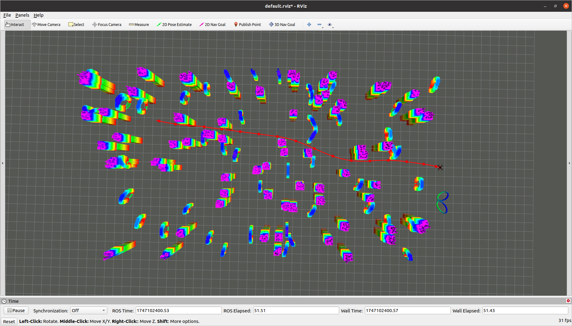
效果展示：

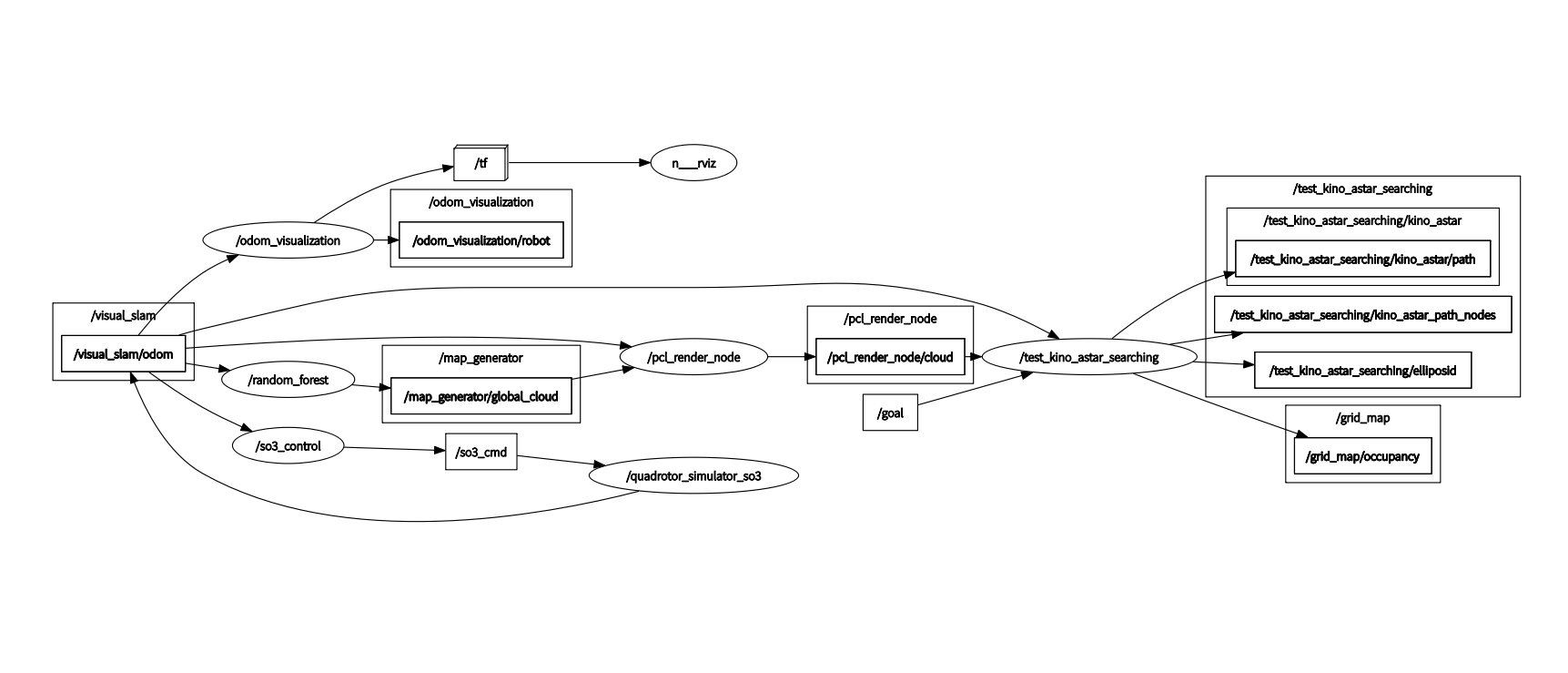
ROS 节点展示全局规划和轨迹生成部分：

Kinodynamic A*代码主体：

int KinoAstar::search(Eigen::Vector3d start_pt, Eigen::Vector3d start_vel,Eigen::Vector3d end_pt, Eigen::Vector3d end_vel,std::vector<Eigen::Vector3d>& path)
{// 记录算法启动时间，计算加速度分辨率倒数，初始化最优时间为无穷大ros::Time start_time = ros::Time::now();double inv_acc_res_ = 1.0 / acc_res_;double optimal_time = inf;// 从节点池中分配起点节点，设置位置、速度、索引、实际代价g_cost（起点到当前节点的累积代价）和综合代价f_cost（g_cost + 启发式代价）KinoAstarNodePtr start_node = path_node_pool_[use_node_num_];start_node->position = start_pt;start_node->velocity = start_vel;start_node->index = posToIndex(start_pt);start_node->g_cost = 0.0;start_node->f_cost = lambda_heu_ * getHeuristicCost(start_pt, start_vel, end_pt, end_vel, optimal_time);use_node_num_++;// 将起点加入优先队列open_list_（按f_cost排序），并标记为“待扩展”open_list_.push(start_node);expanded_list_.insert(start_node->index, start_node);start_node->node_state = IN_OPEN_LIST_;std::vector<Eigen::Vector3d> path_nodes_list;while (!open_list_.empty()){// 循环处理开放列表，取出当前最优节点，移入关闭列表close_list_，标记为“已扩展”KinoAstarNodePtr current_node = open_list_.top();open_list_.pop();close_list_.insert(current_node->index, current_node);current_node->node_state = IN_CLOSE_LIST_;current_node->duration = sample_tau_;// debug// std::cout << "current_node: " << current_node->position.transpose() << std::endl;// check if near goal// 若当前节点接近终点，尝试直接生成无碰撞的最优轨迹（如多项式插值或动力学可行路径）if ((current_node->position - end_pt).norm() < goal_tolerance_){double tmp_cost = lambda_heu_ * getHeuristicCost(current_node->position, current_node->velocity, end_pt, end_vel, optimal_time);bool shot_path_found = computeShotTraj(current_node->position, current_node->velocity, end_pt, end_vel, optimal_time);// std::cout << "optimal_time: " << optimal_time << std::endl;if (shot_path_found){ros::Time end_time = ros::Time::now();std::cout << "kinodynamic path found, time cost: " << (end_time - start_time).toSec() << std::endl;std::cout << "use_node_num: " << use_node_num_ << std::endl;std::cout << "total_cost_J: " << current_node->g_cost + tmp_cost << std::endl;current_node->duration = optimal_time;std::vector<KinoAstarNodePtr> path_pool = retrievePath(current_node, path_nodes_list);path_nodes_list.push_back(end_pt);visPathNodes(path_nodes_list);switch (collision_check_type_){case 1: // grid map check{samplePath(path_pool, path);break;}case 2: // local cloud check{sampleEllipsoid(path_pool, path, rot_list);visEllipsoid(path, rot_list);break;}  }return REACH_END;}else if (current_node->parent != NULL){// std::cout << "near end!" << std::endl;}else{std::cout << "no shot path found, end searching" << std::endl;return NO_PATH_FOUND;   }// else continue;  }// expand current node// (2r+1)^3 samplefor (double ax = -max_accel_; ax <= max_accel_ + 1e-3; ax += inv_acc_res_ * max_accel_)for (double ay = -max_accel_; ay <= max_accel_ + 1e-3; ay += inv_acc_res_ * max_accel_)for (double az = -max_accel_; az <= max_accel_ + 1e-3; az += inv_acc_res_ * max_accel_){Eigen::Vector3d ut;ut << ax, ay, az;Eigen::Matrix<double, 6, 1> x0;x0.head(3) = current_node->position;x0.tail(3) = current_node->velocity;Eigen::Matrix<double, 6, 1> xt;int segment_num = std::floor(sample_tau_ / step_size_);bool flag = false;bool collision_flag = false;for (int i = 0; i <= segment_num; i++){double t = i * step_size_;StateTransit(x0, xt, ut, t);Eigen::Vector3d tmp_pos = xt.head(3);// check collision and if out of mapif (grid_map_->isInMap(tmp_pos) == false){flag = true;break;}// check collisionswitch (collision_check_type_){case 1: // grid map checkif (grid_map_->getInflateOccupancy(tmp_pos) == 1){collision_flag = true;break;}case 2: // local cloud checkif (isCollisionFree(tmp_pos, ut) == false){collision_flag = true;break;}}if (collision_flag){flag = true;break;}// check velocity limitif (xt.tail(3)(0) < -max_vel_ || xt.tail(3)(0) > max_vel_ || xt.tail(3)(1) < -max_vel_ || xt.tail(3)(1) > max_vel_ || xt.tail(3)(2) < -max_vel_ || xt.tail(3)(2) > max_vel_){flag = true;break;}}if (flag) continue;StateTransit(x0, xt, ut, sample_tau_);// std::cout << "xt: " << xt.head(3).transpose() << std::endl;// std::cout << "index: " << posToIndex(xt.head(3)).transpose() << std::endl;// check if in close_list_if (close_list_.find(posToIndex(xt.head(3))) != NULL){continue;}// check if in expanded_list_else if (expanded_list_.find(posToIndex(xt.head(3))) == NULL){KinoAstarNodePtr pro_node = path_node_pool_[use_node_num_];pro_node->position = xt.head(3);pro_node->velocity = xt.tail(3);pro_node->index = posToIndex(xt.head(3));pro_node->g_cost = current_node->g_cost + (ut.dot(ut) + rou_) * sample_tau_;pro_node->f_cost = pro_node->g_cost + lambda_heu_ * getHeuristicCost(pro_node->position, pro_node->velocity, end_pt, end_vel, optimal_time);pro_node->parent = current_node;pro_node->input = ut;pro_node->duration = sample_tau_;pro_node->node_state = IN_OPEN_LIST_;use_node_num_++;open_list_.push(pro_node);expanded_list_.insert(pro_node->index, pro_node);// check if use_node_num reach the max_node_numif (use_node_num_ >= allocated_node_num_){std::cout << "reach max node num, end searching" << std::endl;return NO_PATH_FOUND;}}else{// pruning, if in same grid, check if g_cost is smaller and updatedouble tmp_g_cost = current_node->g_cost + (ut.dot(ut) + rou_) * sample_tau_;KinoAstarNodePtr old_node = expanded_list_.find(posToIndex(xt.head(3)));if (tmp_g_cost < old_node->g_cost){old_node->position = xt.head(3);old_node->velocity = xt.tail(3);// old_node->index = posToIndex(xt.head(3));old_node->g_cost = tmp_g_cost;old_node->f_cost = old_node->g_cost + lambda_heu_ * getHeuristicCost(old_node->position, old_node->velocity, end_pt, end_vel, optimal_time);old_node->parent = current_node;old_node->input = ut;}}}}std::cout << "open_list is empty, end searching, no path found" << std::endl;return NO_PATH_FOUND;
}

 初始化阶段：

ros::Time start_time = ros::Time::now();
double inv_acc_res_ = 1.0 / acc_res_;
double optimal_time = inf;

记录算法启动时间，计算加速度分辨率倒数，初始化最优时间为无穷大。

起点节点初始化：

KinoAstarNodePtr start_node = path_node_pool_[use_node_num_];
start_node->position = start_pt;
start_node->velocity = start_vel;
start_node->index = posToIndex(start_pt);
start_node->g_cost = 0.0;
start_node->f_cost = lambda_heu_ * getHeuristicCost(...);
use_node_num_++;

 从节点池中分配起点节点，设置位置、速度、索引、实际代价g_cost（起点到当前节点的累积代价）和综合代价f_cost（g_cost + 启发式代价）。

开放列表与扩展列表管理​：

open_list_.push(start_node);
expanded_list_.insert(start_node->index, start_node);
start_node->node_state = IN_OPEN_LIST_;

将起点加入优先队列open_list_（按f_cost排序），并标记为“待扩展”。

主搜索循环​:

while (!open_list_.empty()) {
KinoAstarNodePtr current_node = open_list_.top();
open_list_.pop();
close_list_.insert(current_node->index, current_node);
current_node->node_state = IN_CLOSE_LIST_;

循环处理开放列表，取出当前最优节点，移入关闭列表close_list_，标记为“已扩展”。

终点检查与轨迹优化​：

if ((current_node->position - end_pt).norm() < goal_tolerance_) {bool shot_path_found = computeShotTraj(...);if (shot_path_found) {samplePath(path_pool, path);return REACH_END;}
}

若当前节点接近终点，尝试直接生成无碰撞的最优轨迹（如多项式插值或动力学可行路径）。

samplePath：

主体部分：

void KinoAstar::samplePath(std::vector<KinoAstarNodePtr> path_pool, std::vector<Eigen::Vector3d>& path)
{// 当路径池中有多个节点时（非单节点情况）if (path_pool.size() != 1){// 遍历路径池中相邻的节点对for (int i = 0; i < path_pool.size() - 1; i++){KinoAstarNodePtr curr_node = path_pool[i];   // 当前路径节点KinoAstarNodePtr next_node = path_pool[i + 1]; // 下一路径节点double curr_t = 0.0;  // 当前时间戳Eigen::Matrix<double, 6, 1> x0, xt; // 状态向量（6维：位置+速度）x0 << curr_node->position, curr_node->velocity; // 初始化当前状态// 根据节点持续时间分割时间段（基于固定步长step_size_）int segment_num = std::floor(curr_node->duration / step_size_);// 逐时间段生成路径点for (int j = 0; j < segment_num; j++){curr_t = j * step_size_;  // 计算当前时间StateTransit(x0, xt, next_node->input, curr_t); // 状态转移计算（可能涉及运动学方程）[1,5](@ref)path.push_back(xt.head(3));  // 将位置信息(x,y,z)加入路径集合}// 处理最后一个时间段（可能不完整的步长）StateTransit(x0, xt, next_node->input, curr_node->duration);// 验证最终状态与目标节点的位置一致性if ((xt.head(3) - next_node->position).norm() > 1e-2){std::cerr << "error in sample!" << std::endl; // 超阈值报错}}// 处理路径池中最后一个节点的轨迹KinoAstarNodePtr last_node = path_pool.back();double td = last_node->duration;  // 获取总持续时间Eigen::Matrix<double, 4, 1> t_vector; // 时间多项式向量（t^0, t^1, t^2, t^3）// 分割时间段生成路径点int segment_num = std::floor(td / step_size_);double curr_t = 0.0;for (int j = 0; j <= segment_num; j++){curr_t = j * step_size_;  // 当前时间戳for (int i = 0; i < 4; i++) {t_vector(i) = pow(curr_t, i); // 构建时间多项式项（如t³, t², t, 1）}Eigen::Vector3d shot_pos = shot_coef_ * t_vector; // 通过多项式系数生成路径点（轨迹插值）[5](@ref)path.push_back(shot_pos); // 将插值点加入路径}}else  // 当路径池只有单个节点时的处理逻辑{KinoAstarNodePtr last_node = path_pool.back();double td = last_node->duration;  // 总持续时间Eigen::Matrix<double, 4, 1> t_vector; // 同上时间多项式向量int segment_num = std::floor(td / step_size_);double curr_t = 0.0;for (int j = 0; j <= segment_num; j++) {curr_t = j * step_size_;for (int i = 0; i < 4; i++) {t_vector(i) = pow(curr_t, i);}Eigen::Vector3d shot_pos = shot_coef_ * t_vector; // 多项式轨迹生成path.push_back(shot_pos);}}
}

 该函数主要用于：

1. ​​路径采样​​：根据路径池（path_pool）中的节点，通过时间分片（step_size_）生成连续路径点。
2. ​​状态转移​​：在多节点情况下，通过StateTransit函数计算相邻节点间的运动状态（可能包含速度/加速度模型）
3. ​​轨迹插值​​：在单节点或最终阶段，利用四次多项式系数（shot_coef_）生成平滑轨迹，适用于机器人/自动驾驶的运动规划
4. ​​错误校验​​：检查采样结果与目标节点的位置偏差，确保路径精度。

getHeuristicCost：

主体部分：

double KinoAstar::getHeuristicCost(Eigen::Vector3d x1, Eigen::Vector3d v1,Eigen::Vector3d x2, Eigen::Vector3d v2,double &optimal_time)
{Eigen::Vector3d dp = x2 - x1;double optimal_cost = inf;double a = -36 * dp.dot(dp);double b = 24 * dp.dot(v1 + v2);double c = -4 * (v1.dot(v1) + v1.dot(v2) + v2.dot(v2));double d = 0;double e = rou_;std::vector<double> dts = quartic(e, d, c, b, a);double T_bar = ((x1 - x2).lpNorm<Eigen::Infinity>() / max_vel_);for (int i = 0; i < dts.size(); i++){double t = dts[i];double tmp_cost = a / (-3 * t * t * t) + b / (-2 * t * t) + c / (-1 * t) + e * t;if (tmp_cost < optimal_cost && t > T_bar && tmp_cost > 0){optimal_cost = tmp_cost;optimal_time = t;}}return tie_breaker_ * optimal_cost;}

 KinoAstar::getHeuristicCost 是运动规划中结合动力学约束的启发式函数，其核心目标是​​通过最优控制理论计算从当前状态到目标状态的最小控制能量代价​​，用于引导A*算法的搜索方向并加速收敛。以下是逐层解析：

函数参数与目标​：

• 输入参数​​：
  • x1/v1：起点位置和速度
  • x2/v2：终点位置和速度
  • optimal_time（输出）：最优时间估计
• ​​输出​​：启发式代价（预估最小控制能量）

 数学原理：最优控制问题建模​：

​该函数基于​​庞特里亚金极小值原理​​（Pontryagin's Minimum Principle），求解两点边界最优控制问题（OBVP）。目标是最小化控制能量（如加加速度的积分），同时满足位置和速度的终点约束。

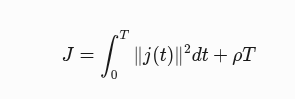
其中：

• j(t) 是加加速度（控制输入）
• ρ 是时间权重（对应代码中的 rou_）

通过状态方程和协态方程推导，最终得到关于时间 T 的​​四次多项式方程​​，其根对应可能的极值点。

代码实现步骤​：

1. 构造四次方程系数​​：

   • 计算位置差 dp = x2 - x1
   • 根据几何关系和控制能量积分，生成系数 a, b, c, d, e（对应四次方程 aT^4+bT^3+cT^2+d^T+e=0）

2. ​​求解方程根​​：

   • 调用 quartic(e, d, c, b, a) 解四次方程，得到候选时间解 dts。

3. ​​筛选最优时间与代价​​：

   • 计算时间下限 T_bar（确保速度不超过最大值 max_vel_）
   • 遍历所有候选时间 t，计算对应的能量代价 tmp_cost，筛选满足 t>T_bar 的最小代价 optimal_cost 及对应时间 optimal_time。

4. ​​返回加权代价​​：

   • 最终代价乘以 tie_breaker_（通常略大于1的系数，避免路径重复扩展）

computeShotTraj：

主体部分：

bool KinoAstar::computeShotTraj(Eigen::Vector3d x1, Eigen::Vector3d v1,Eigen::Vector3d x2, Eigen::Vector3d v2,double optimal_time)
{double td = optimal_time;Eigen::Vector3d dp = x2 - x1;Eigen::Vector3d dv = v2 - v1;shot_coef_.col(0) = x1;shot_coef_.col(1) = v1;shot_coef_.col(2) = 0.5 * (6 / (td * td) * (dp - v1 * td) - 2 * dv / td);shot_coef_.col(3) = 1.0 / 6.0 * (-12 / (td * td *td) * (dp - v1 * td) + 6 * dv / (td * td));Eigen::Matrix<double, 4, 4> Transit_v;Transit_v << 0, 0, 0, 0, 1, 0, 0, 0,0, 2, 0, 0, 0, 0, 3, 0;Eigen::Matrix<double, 4, 4> Transit_a;Transit_a << 0, 0, 0, 0, 1, 0, 0, 0,0, 2, 0, 0, 0, 0, 0, 0;vel_coef_ = shot_coef_ * Transit_v;acc_coef_ = vel_coef_ * Transit_a;Eigen::Matrix<double, 4, 1> t_vector;int segment_num = std::floor(td / step_size_);double curr_t = 0.0;for (int j = 0; j <= segment_num; j++){curr_t = j * step_size_;for (int i = 0; i < 4; i++){t_vector(i) = pow(curr_t, i);}Eigen::Vector3d shot_pos = shot_coef_ * t_vector;Eigen::Vector3d shot_vel = vel_coef_ * t_vector;Eigen::Vector3d shot_acc = acc_coef_ * t_vector;// check collisionif (grid_map_->getInflateOccupancy(shot_pos)){return false;}// only check collision, vel and acc limit by limit T_// // check velocity limit// if (shot_vel(0) > max_vel_ || shot_vel(0) < -max_vel_ || //     shot_vel(1) > max_vel_ || shot_vel(1) < -max_vel_ || //     shot_vel(2) > max_vel_ || shot_vel(2) < -max_vel_)// {//   return false;// }// // check acceleration limit// if (shot_acc(0) > max_accel_ || shot_acc(0) < -max_accel_ || //     shot_acc(1) > max_accel_ || shot_acc(1) < -max_accel_ || //     shot_acc(2) > max_accel_ || shot_acc(2) < -max_accel_)// {//   return false;// }}return true;
}

 定义了一个函数computeShotTraj，属于类KinoAstar：

bool KinoAstar::computeShotTraj(Eigen::Vector3d x1, Eigen::Vector3d v1,Eigen::Vector3d x2, Eigen::Vector3d v2,double optimal_time)

 该函数用于计算一步到位的航迹，参数包括初始位置x1、初始速度v1、目标位置x2、目标速度v2，以及最优时间optimal_time，返回值为布尔类型。

double td = optimal_time;

将optimal_time赋值给变量td，表示轨迹的时间长度。

Eigen::Vector3d dp = x2 - x1;
Eigen::Vector3d dv = v2 - v1;

计算位置差和速度差。

shot_coef_.col(0) = x1;
shot_coef_.col(1) = v1;
shot_coef_.col(2) = 0.5 * (6 / (td * td) * (dp - v1 * td) - 2 * dv / td);
shot_coef_.col(3) = 1.0 / 6.0 * (-12 / (td * td *td) * (dp - v1 * td) + 6 * dv / (td * td));

 将初始位置x1和初始速度v1赋值给shot_coef_的第一列和第二列，shot_coef_是一个用于存储三次多项式系数的矩阵。计算三次多项式的第二项系数，涉及位置差dp、初始速度v1、速度差dv，以及时间td的计算。

Eigen::Matrix<double, 4, 4> Transit_v;Transit_v << 0, 0, 0, 0, 1, 0, 0, 0,0, 2, 0, 0, 0, 0, 3, 0;Eigen::Matrix<double, 4, 4> Transit_a;Transit_a << 0, 0, 0, 0, 1, 0, 0, 0,0, 2, 0, 0, 0, 0, 0, 0;

定义一个4x4的矩阵Transit_v，用于将位置系数转换为速度系数。矩阵的结构是根据速度的导数特性定义的。定义一个4x4的矩阵Transit_a，用于将速度系数转换为加速度系数。矩阵的结构是根据加速度的导数特性定义的。

vel_coef_ = shot_coef_ * Transit_v;
acc_coef_ = vel_coef_ * Transit_a;

通过shot_coef_和Transit_v的矩阵乘法，计算出速度系数矩阵vel_coef_。 通过vel_coef_和Transit_a的矩阵乘法，计算出加速度系数矩阵acc_coef_。

Eigen::Matrix<double, 4, 1> t_vector;
int segment_num = std::floor(td / step_size_);
double curr_t = 0.0;
for (int j = 0; j <= segment_num; j++){curr_t = j * step_size_;for (int i = 0; i < 4; i++){t_vector(i) = pow(curr_t, i);}Eigen::Vector3d shot_pos = shot_coef_ * t_vector;Eigen::Vector3d shot_vel = vel_coef_ * t_vector;Eigen::Vector3d shot_acc = acc_coef_ * t_vector;// check collisionif (grid_map_->getInflateOccupancy(shot_pos)){return false;}

 定义一个4x1的矩阵t_vector，用于存储时间的幂次计算。计算时间分割数segment_num，即时间td除以步长step_size_并向下取整。循环遍历时间分割点，从0到segment_num。计算当前时间curr_t，即j乘以步长step_size_。通过shot_coef_和t_vector的矩阵乘法，计算出当前位置shot_pos。通过vel_coef_和t_vector的矩阵乘法，计算出当前速度shot_vel。通过acc_coef_和t_vector的矩阵乘法，计算出当前加速度shot_acc。检查当前位置shot_pos是否与网格地图中的膨胀障碍物发生碰撞。如果发生碰撞，返回false，表示轨迹不可行。

retrievePath：

主体部分：

std::vector<KinoAstarNodePtr> KinoAstar::retrievePath(KinoAstarNodePtr end_node, std::vector<Eigen::Vector3d>& path_nodes_list)
{KinoAstarNodePtr current_node = end_node;std::vector<KinoAstarNodePtr> path_nodes;while (current_node->parent != NULL){path_nodes.push_back(current_node);path_nodes_list.push_back(current_node->position);current_node = current_node->parent;}path_nodes.push_back(current_node);path_nodes_list.push_back(current_node->position);std::reverse(path_nodes.begin(), path_nodes.end());std::reverse(path_nodes_list.begin(), path_nodes_list.end());return path_nodes;
}

std::vector<KinoAstarNodePtr> path_pool = retrievePath(current_node, path_nodes_list);

这段代码定义了一个函数 retrievePath，属于类 KinoAstar，用于从终点节点回溯并提取出路径上的所有节点以及它们的位置，形成完整的路径。

1. 路径回溯：从终点节点开始，通过每个节点的parent指针逐级向上访问，直到找到起点（即parent为NULL的节点）。
2. 路径构建：在回溯过程中，将每个节点及其位置分别添加到path_nodes和path_nodes_list中。
3. 顺序调整：由于回溯得到的路径是从终点到起点的顺序，使用std::reverse将两个向量反转，最终得到从起点到终点的正确路径顺序。

 节点扩展与状态转移：

for (double ax = -max_accel_; ...) {Eigen::Vector3d ut(ax, ay, az);StateTransit(x0, xt, ut, sample_tau_);// 碰撞检测与速度限制检查
}

 功能​​：遍历所有可能的加速度控制输入（三维离散化），生成子节点状态

• 关键点​​：
  • ​​状态转移方程​​：StateTransit根据动力学模型（如匀加速运动学）计算下一时刻状态
  • ​​碰撞检测​​：分段检查轨迹段是否在自由空间内（grid_map_或点云检测）

StateTransit： 

主体部分：

void KinoAstar::StateTransit(Eigen::Matrix<double, 6, 1> &x0, Eigen::Matrix<double, 6, 1> &xt,Eigen::Vector3d ut, double t)
{// 初始化6x6状态转移矩阵e_At为单位矩阵（初始状态下时间t=0时的状态转移）Eigen::Matrix<double, 6, 6> e_At = Eigen::Matrix<double, 6, 6>::Identity();// 前三行的位置-速度关系处理：位置 += 速度 * 时间t（例如x = x0 + vx*t）for (int i = 0; i < 3; i++) {e_At(i, 3 + i) = t;  // 例如e_At矩阵第0行第3列设为t，对应x方向的位置增量}// 初始化6x3的积分矩阵（用于控制输入ut对状态的影响）Eigen::Matrix<double, 6, 3> Integral = Eigen::Matrix<double, 6, 3>::Zero();// 填充积分矩阵：// 前三行对角线元素为0.5*t²（加速度对位置的影响，如Δx = 0.5*a*t²）// 后三行对角线元素为t（加速度对速度的影响，如Δv = a*t）for (int i = 0; i < 6; i++) {if (i < 3) Integral(i, i) = 0.5 * t * t;  // 位置积分项else Integral(i, i - 3) = t;         // 速度积分项}// 状态转移方程：xt = e_At * x0 + Integral * ut// 其中：// - e_At * x0 表示初始状态的线性传播（位置+速度）// - Integral * ut 表示控制输入（如加速度）对状态的影响xt = e_At * x0 + Integral * ut;
}

功能总结：

1. ​​状态转移模型​​
   基于线性运动学模型，通过矩阵运算实现状态预测。假设系统为二阶模型（包含位置和速度），控制输入ut可能对应加速度

2. ​​矩阵作用​​

   • ​​e_At​​：6x6矩阵，描述位置和速度随时间变化的线性关系（如匀速运动模型）。
   • ​​Integral​​：6x3矩阵，计算控制输入对状态的积分贡献（如匀加速运动中的位移和速度变化）

3. ​​物理意义​​
   假设系统状态为[x, y, z, vx, vy, vz]，控制输入为加速度[ax, ay, az]，则：

   • 位置更新：x_new = x0 + vx*t + 0.5*ax*t²
   • 速度更新：vx_new = vx + ax*t