使用Mathematica绘制Peano Curve

皮亚诺（Peano）曲线，是一条可以填充平面的曲线。在Mathematica中，内置了函数PeanoCurve，可以用来绘制不同深度的皮亚诺曲线。这个函数，返回的是一个Line对象，为一串折线，可以使用Graphics函数，将相应图形绘制出来。

使用如下代码：

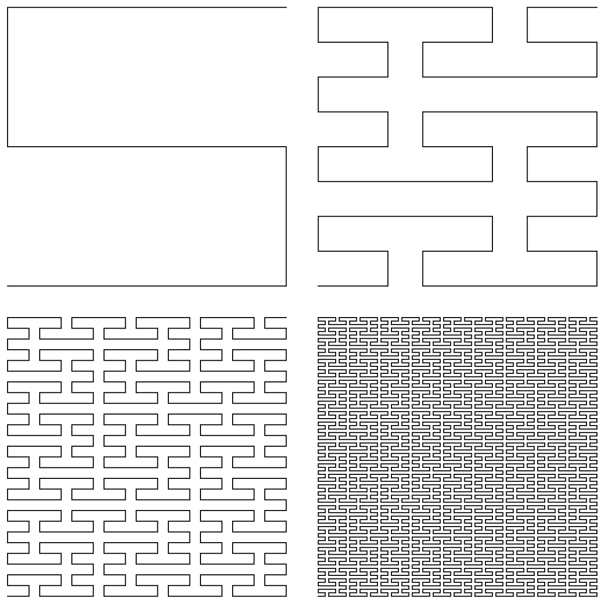
GraphicsGrid[ { {Graphics[PeanoCurve[1]], Graphics[PeanoCurve[2]]}, {Graphics[PeanoCurve[3]], Graphics[PeanoCurve[4]]} } ]

可以得到如下对比图案：

可以通过DataRange指定坐标范围。

Graphics[ PeanoCurve[3, DataRange -> {{0, 1}, {0, 1}}], PlotRange -> 2, Axes -> True ]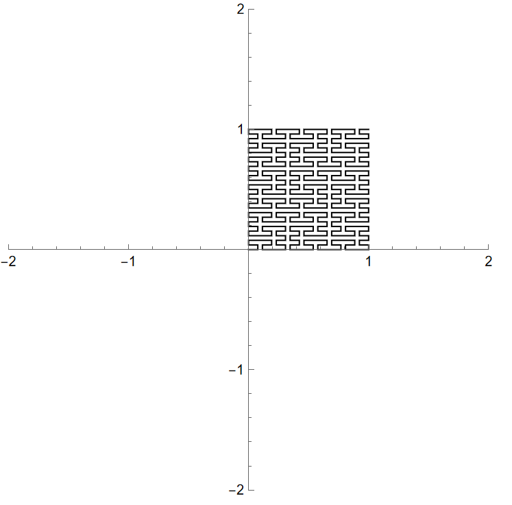

指定坐标范围之后，可以使用BSplineFuntion将Line对象，转成参数函数。

BSplineFunction[PeanoCurve[3, DataRange -> {{-1, 1}, {-1, 1}}][[1]], SplineDegree -> 1]; ParametricPlot[%[t], {t, 0, 1}, PlotPoints -> 400]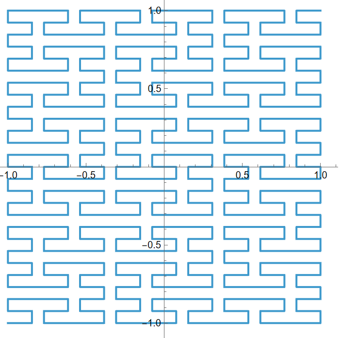

在Mathematica中，这种转化方式，也灵活多变，比如，也可以采用如下方式：

Graphics[ { Thickness[Large], PeanoCurve[3] /. Line -> BSplineCurve } ]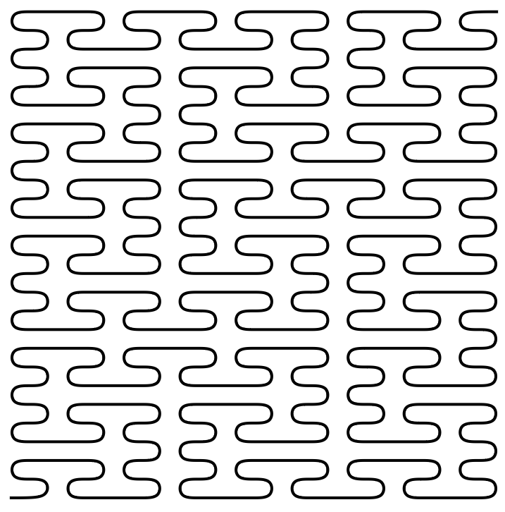

有了这样的参数化之后，就很容易来做绘制过程了：

tempFunc00 = BSplineFunction[PeanoCurve[6, DataRange -> {{-1, 1}, {-1, 1}}][[1]], SplineDegree -> 1]; Animate[ParametricPlot[tempFunc00[t], {t, 0, n}, PlotPoints -> 400, PlotRange -> {{-1, 1}, {-1, 1}}], {n, 0.01, 1, 0.01}]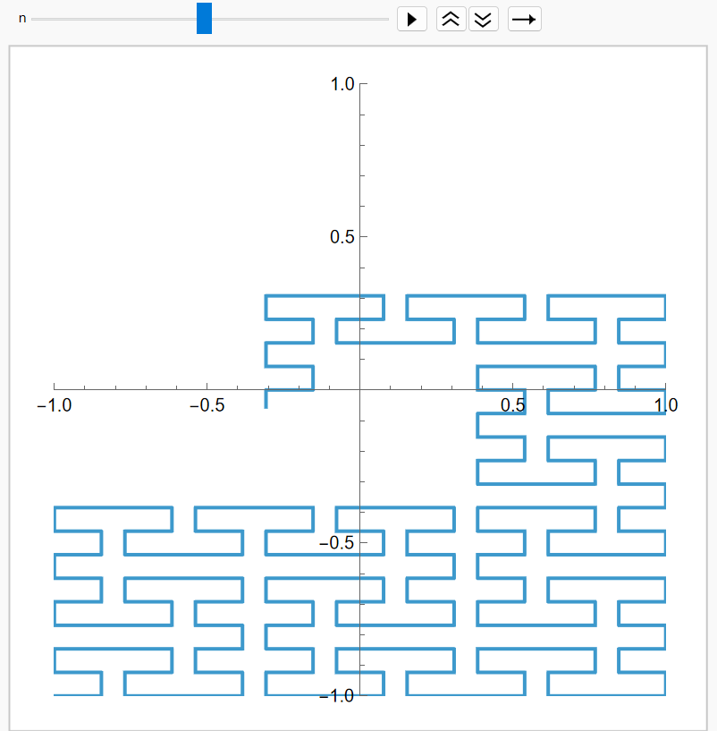

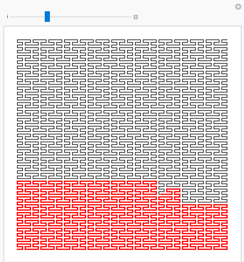
上面的动画效果，也可以不是用BSplineFunction的参数化，而直接使用Line对象的前面i段，来实现动态效果。

With[ {curve = PeanoCurve[4]}, Manipulate[ Graphics[ {curve, Red, Thick, Line[ Take[First[curve], i] ] }, ImageSize -> Medium ], {i, 1, 6561, 1} ] ]