注意力机制

注意力机制

心理学

动物需要在复杂的环境下有效关注值得注意的点
心理学框架：人类根据随意线索和不随意线索选择注意点

红色杯子：不随意线索（红色的杯子比较的显著，不需要额外的想法，自然而然会去看这个）

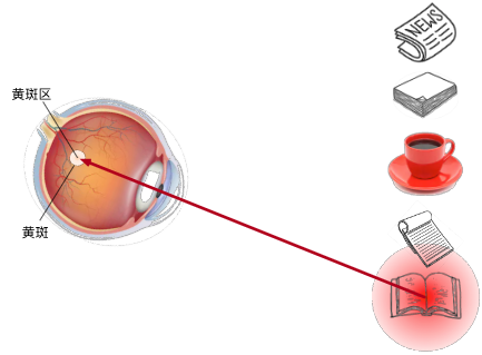
想读书：随意线索

注意力机制

卷积、全连接、池化层都只考虑不随意线索
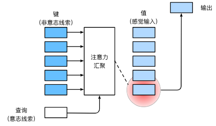
注意力机制则显示的考虑随意线索

• 随意线索被称之为查询（query）
• 每个输入是一个值（value）和不随意线索（key）的对
• 通过注意力池化层来有偏向性的选择某些输入

非参注意力池化层

• 给定数据 $(x_i,y_i),i=1,...,n$
• 平均池化是最简单的方案：$f(x)=\frac{1}{n}{\sum }_i{y}_i$
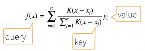
• 更好的方案是 60 年代提出来的 Nadaraya-Watson 核回归

$f(x)={\sum }_{i=1}^n\frac{K(x-x_i)}{{\sum }_{j=1}^{n}K(x-x_j)}{y}_i$

Nadaraya-Watson核回归

• 使用高斯核 $K(u)=\frac{1}{\sqrt{2\pi }}\exp (-\frac{u^2}{2})$
• 那么 $f(x)={\sum }_{i=1}^n\frac{\exp \left(-\frac{1}{2}(x-x_i{)}^2\right)}{{\sum }_{j=1}^n\exp \left(-\frac{1}{2}(x-x_j{)}^2\right)}{y}_i$
  $={\sum }_{i=1}^n\text{softmax}\left(-\frac{1}{2}(x-x_i{)}^2\right)y_i$

参数化的注意力机制

在之前基础上引入可以学习的 $w$
$f(x)={\sum }_{i=1}^n\text{softmax}\left(-\frac{1}{2}((x-x_i)w{)}^2\right)y_i$

总结

• 心理学认为人通过随意线索和不随意线索选择注意点
• 注意力机制中，通过query（随意线索）和key（不随意线索）来有偏向性的选择输入
  • 可以一般的写作 $f(x)={\sum }_i\alpha (x,x_i)y_i$，这里 $\alpha (x,x_i)$ 是注意力权重
  • 早在60年代就有非参数的注意力机制
  • 下面介绍多个不同的权重设计

代码实现

注意力汇聚：Nadaraya - Watson 核回归

import torch
from torch import nn
from d2l import torch as d2l

生成数据集

n_train = 50  # 训练样本数
x_train, _ = torch.sort(torch.rand(n_train) * 5)   # 排序后的训练样本def f(x):return 2 * torch.sin(x) + x**0.8y_train = f(x_train) + torch.normal(0.0, 0.5, (n_train,))  # 训练样本的输出
x_test = torch.arange(0, 5, 0.1)  # 测试样本
y_truth = f(x_test)  # 测试样本的真实输出
n_test = len(x_test)  # 测试样本数
n_test

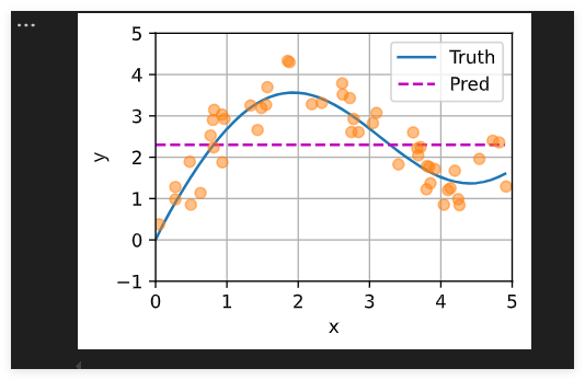
可视化看一下

def plot_kernel_reg(y_hat):d2l.plot(x_test, [y_truth, y_hat], 'x', 'y', legend=['Truth', 'Pred'],xlim=[0, 5], ylim=[-1, 5])d2l.plt.plot(x_train, y_train, 'o', alpha=0.5);y_hat = torch.repeat_interleave(y_train.mean(), n_test)
plot_kernel_reg(y_hat)

非参数注意力汇聚

# X_repeat的形状:(n_test,n_train),
# 每一行都包含着相同的测试输入（例如：同样的查询）
X_repeat = x_test.repeat_interleave(n_train).reshape((-1, n_train))
# x_train包含着键。attention_weights的形状：(n_test,n_train),
# 每一行都包含着要在给定的每个查询的值（y_train）之间分配的注意力权重
attention_weights = nn.functional.softmax(-(X_repeat - x_train)**2 / 2, dim=1)
# y_hat的每个元素都是值的加权平均值，其中的权重是注意力权重
y_hat = torch.matmul(attention_weights, y_train)
plot_kernel_reg(y_hat)

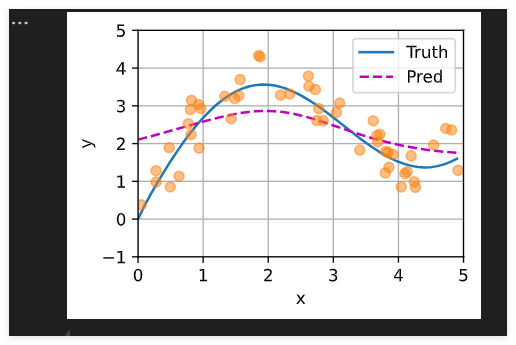
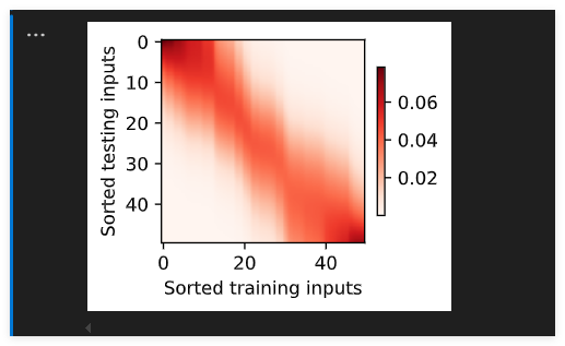
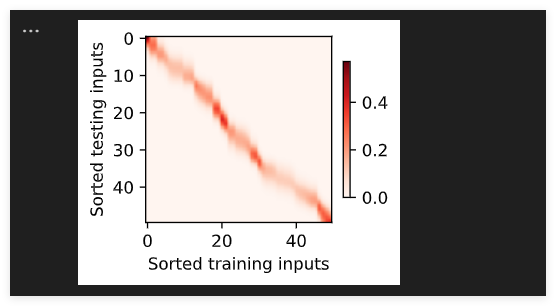
注意力权重

d2l.show_heatmaps(attention_weights.unsqueeze(0).unsqueeze(0),xlabel='Sorted training inputs',ylabel='Sorted testing inputs')

带参数注意力汇聚 假定两个张量的形状分别是 $(n,a,b)$ 和 $(n,b,c)$，它们的批量矩阵乘法输出的形状为 $(n,a,c)$

X = torch.ones((2, 1, 4))
Y = torch.ones((2, 4, 6))
torch.bmm(X, Y).shape# torch.Size([2, 1, 6])

带参数的注意力汇聚

class NWKernelRegression(nn.Module):def __init__(self, **kwargs):super().__init__(**kwargs)self.w = nn.Parameter(torch.rand((1,), requires_grad=True))def forward(self, queries, keys, values):# queries和attention_weights的形状为(查询个数，“键－值”对个数)queries = queries.repeat_interleave(keys.shape[1]).reshape((-1, keys.shape[1]))self.attention_weights = nn.functional.softmax(-((queries - keys) * self.w)**2 / 2, dim=1)# values的形状为(查询个数，“键－值”对个数)return torch.bmm(self.attention_weights.unsqueeze(1),values.unsqueeze(-1)).reshape(-1)

将训练数据集转换为键和值

# X_tile的形状:(n_train，n_train)，每一行都包含着相同的训练输入
X_tile = x_train.repeat((n_train, 1))
# Y_tile的形状:(n_train，n_train)，每一行都包含着相同的训练输出
Y_tile = y_train.repeat((n_train, 1))
# keys的形状:('n_train'，'n_train'-1)
keys = X_tile[(1 - torch.eye(n_train)).type(torch.bool)].reshape((n_train, -1))
# values的形状:('n_train'，'n_train'-1)
values = Y_tile[(1 - torch.eye(n_train)).type(torch.bool)].reshape((n_train, -1))

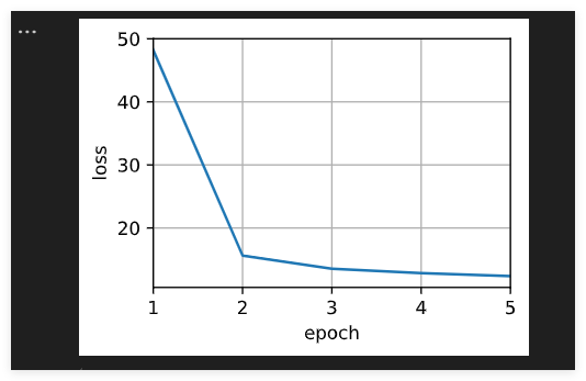
训练带参数的注意力汇聚模型

net = NWKernelRegression()
loss = nn.MSELoss(reduction='none')
trainer = torch.optim.SGD(net.parameters(), lr=0.5)
animator = d2l.Animator(xlabel='epoch', ylabel='loss', xlim=[1, 5])for epoch in range(5):trainer.zero_grad()l = loss(net(x_train, keys, values), y_train)l.sum().backward()trainer.step()print(f'epoch {epoch + 1}, loss {float(l.sum()):.6f}')animator.add(epoch + 1, float(l.sum()))

预测结果绘制

# keys的形状:(n_test，n_train)，每一行包含着相同的训练输入（例如，相同的键）
keys = x_train.repeat((n_test, 1))
# value的形状:(n_test，n_train)
values = y_train.repeat((n_test, 1))
y_hat = net(x_test, keys, values).unsqueeze(1).detach()
plot_kernel_reg(y_hat)

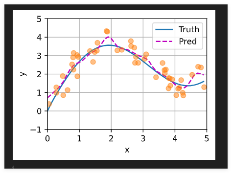
曲线在注意力权重较大的区域变得更不平滑

d2l.show_heatmaps(net.attention_weights.unsqueeze(0).unsqueeze(0),xlabel='Sorted training inputs',ylabel='Sorted testing inputs')

小结

• Nadaraya-Watson核回归是具有注意力机制的机器学习范例。
• Nadaraya-Watson核回归的注意力汇聚是对训练数据中输出的加权平均。从注意力的角度来看，分配给每个值的注意力权重取决于将值所对应的键和查询作为输入的函数。
• 注意力汇聚可以分为非参数型和带参数型。