当前位置：首页 > news >正文

[machine learning] Transformer - Attention (一)

news 来源：原创 2025/5/3 6:20:28

Attention是Transformer的核心，本系列先通过介绍Attention来学习Transformer。本文先介绍简单版的Attention。

在Attention出现之前，通常使用recurrent neural networds (RNNs)来处理长序列数据。模型架构上，又通常使用encoder-decoder的结构。
以机器翻译为例，当输入文本序列一个一个进入encoder时，encoder也在一步一步地更新它的hidden state(即隐藏层的值)。通过这种方式，encoder在最后一次更新完hidden state后，尽可能多地把整个输入文本序列的含义捕捉存储到最终的hidden state中。decoder以encoder的最终hidden state作为输入，一次一个字地开始翻译。同样，decoder也是一步一步地更新它的hidden state，每一次更新后的hidden state都包含了预测下一个字的必要上下文信息。下面的图就是整个流程：
在这里插入图片描述
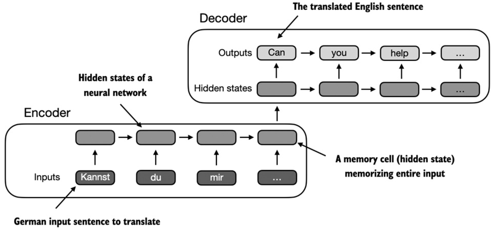
整个流程的关键点是encoder将整个文本序列处理成最终的hidden state(memory cell)。decoder以encoder最终的hidden state为输入，生成输出。encoder-decoder RNN架构最大的问题和局限性是在decoding阶段，RNN无法直接访问encoder中比较靠前的hidden state。结果decoder只能基于包含了所有相关信息的最终hidden state。当遇到复杂的前后依赖距离跨度大的长句时，这个问题会导致上下文信息的丢失。

Transformer的提出解决了RNN的缺陷并逐渐取代了RNN在NLP领域的位置。而Transformer的核心正是self-attention。self-attention是这样一套机制，当计算一个序列的表示时，它允许序列中每个位置上的元素去关注序列中其他位置(包括它本身)的元素。self-attention中的"self"是指这套机制能够通过比较当前位置元素与其他所有位置元素的相关性来计算出关注度权重(attention weights)。它评估学习了输入自己本身不同部分之间的联系和依赖关系。

有了上面的基本概念之后，下面先看一个没有训练权重的simple self-attention。

假设现在有一个6个单词的序列，每个单词的embedding维度是3。

import torch
inputs = torch.tensor(
[[0.43, 0.15, 0.89], # Your (x^1)
[0.55, 0.87, 0.66], # journey (x^2)
[0.57, 0.85, 0.64], # starts (x^3)
[0.22, 0.58, 0.33], # with (x^4)
[0.77, 0.25, 0.10], # one (x^5)
[0.05, 0.80, 0.55]] # step (x^6)
)

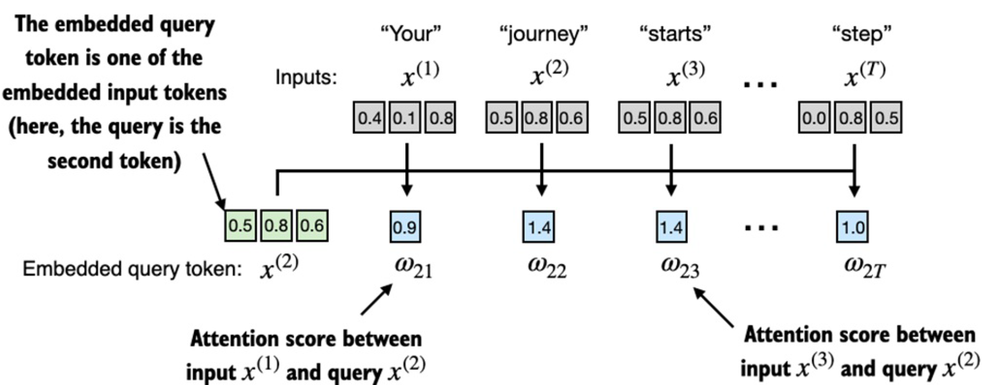
现在我们想要计算第二个单词跟其他所有单词的attention weight。首先我们先计算attention score:

query = inputs[1]
attn_scores_2 = torch.empty(inputs.shape[0])
for i, x_i in enumerate(inputs):attn_scores_2[i] = torch.dot(x_i, query)
print(attn_scores_2)
# 输出：
# tensor([0.9544, 1.4950, 1.4754, 0.8434, 0.7070, 1.0865])

这里我们使用的点乘(dot product)。点乘是将两个向量element-wise地相乘然后相加。点乘结果越大表明两个向量越相关。这部分过程如下图所示：
在这里插入图片描述
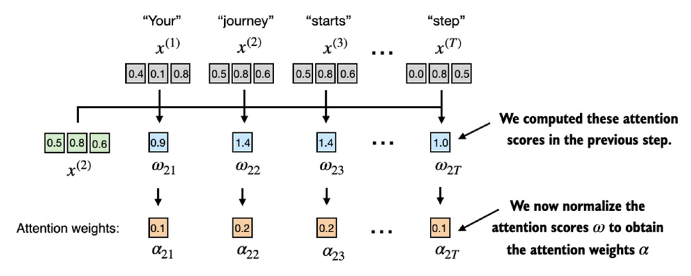
接下来，我们对attention score做归一化求attention weight。

attn_weights_2_tmp = attn_scores_2 / attn_scores_2.sum()
print("Attention weights:", attn_weights_2_tmp)
print("Sum:", attn_weights_2_tmp.sum())
# 输出：
# Attention weights: tensor([0.1455, 0.2278, 0.2249, 0.1285, 0.1077, 0.1656])
# Sum: tensor(1.0000)

实际中，主要是用PyTorch自带的softmax函数来做这个归一化：

attn_weights_2 = torch.softmax(attn_scores_2, dim=0)
print("Attention weights:", attn_weights_2)
print("Sum:", attn_weights_2.sum())
# 输出：
# Attention weights: tensor([0.1385, 0.2379, 0.2333, 0.1240, 0.1082, 0.1581])
# Sum: tensor(1.)

在这里插入图片描述

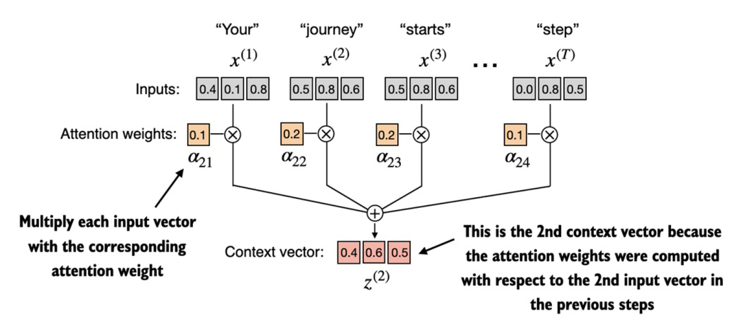
有了attention weight之后，就是最后一步，求第二个单词的上下文向量。

query = inputs[1] # 2nd input token is the query
context_vec_2 = torch.zeros(query.shape)
for i,x_i in enumerate(inputs):
context_vec_2 += attn_weights_2[i]*x_i
print(context_vec_2)
# 输出：
# tensor([0.4419, 0.6515, 0.5683])

在这里插入图片描述

上面是计算第二个单词的上下文向量，下面我们一次性地求所有单词的上下文向量：

# @ 是矩阵乘法，inputs.T 是转置操作
attn_scores = inputs @ inputs.T
print(attn_scores)
# tensor([[0.9995, 0.9544, 0.9422, 0.4753, 0.4576, 0.6310],
# [0.9544, 1.4950, 1.4754, 0.8434, 0.7070, 1.0865],
# [0.9422, 1.4754, 1.4570, 0.8296, 0.7154, 1.0605],
# [0.4753, 0.8434, 0.8296, 0.4937, 0.3474, 0.6565],
# [0.4576, 0.7070, 0.7154, 0.3474, 0.6654, 0.2935],
# [0.6310, 1.0865, 1.0605, 0.6565, 0.2935, 0.9450]])# 注意在第一维上做softmax
attn_weights = torch.softmax(attn_scores, dim=1)
print(attn_weights)
# 可以看到每一行加起来都是1
# tensor([[0.2098, 0.2006, 0.1981, 0.1242, 0.1220, 0.1452],
# [0.1385, 0.2379, 0.2333, 0.1240, 0.1082, 0.1581],
# [0.1390, 0.2369, 0.2326, 0.1242, 0.1108, 0.1565],
# [0.1435, 0.2074, 0.2046, 0.1462, 0.1263, 0.1720],
# [0.1526, 0.1958, 0.1975, 0.1367, 0.1879, 0.1295],
# [0.1385, 0.2184, 0.2128, 0.1420, 0.0988, 0.1896]])all_context_vecs = attn_weights @ inputs
print(all_context_vecs)
# tensor([[0.4421, 0.5931, 0.5790],
# [0.4419, 0.6515, 0.5683],
# [0.4431, 0.6496, 0.5671],
# [0.4304, 0.6298, 0.5510],
# [0.4671, 0.5910, 0.5266],
# [0.4177, 0.6503, 0.5645]])