当前位置：首页 > news >正文

基于CT成像的肿瘤图像分类：方法与实现

news 来源：原创 2025/4/30 17:55:44

引言

医学影像分析是现代医疗诊断中不可或缺的一部分，其中计算机断层扫描(CT)成像技术在肿瘤检测和诊断中发挥着重要作用。随着深度学习技术的快速发展，基于CT图像的自动肿瘤分类系统已成为研究热点。本文将详细介绍如何使用深度学习技术对CT图像中的肿瘤进行分类，并提供完整的代码实现。

一、CT图像与肿瘤诊断

1.1 CT成像技术概述

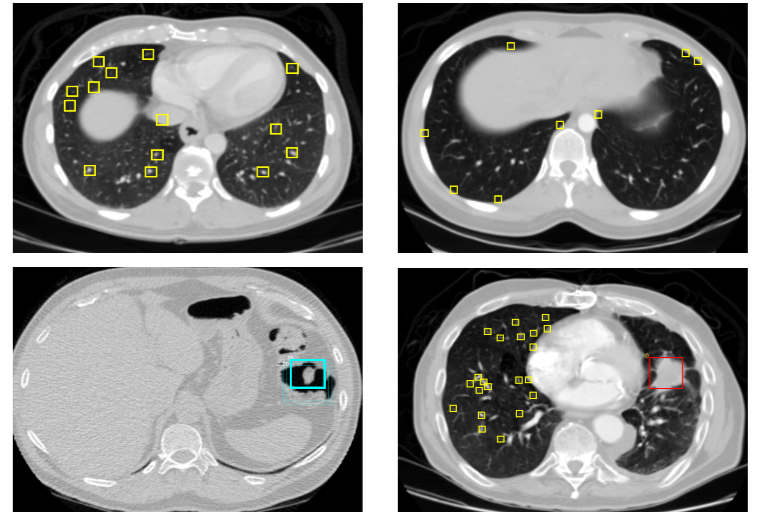
计算机断层扫描(CT)是通过X射线旋转扫描人体部位，由计算机重建出横断面图像的成像技术。与普通X光片相比，CT能提供更详细的解剖结构信息，具有更高的密度分辨率，能够清晰显示软组织间的差异。

1.2 肿瘤在CT图像中的表现

不同类型的肿瘤在CT图像上表现出不同的特征：

良性肿瘤：通常边界清晰、形态规则、密度均匀
恶性肿瘤：往往边界模糊、形态不规则、密度不均匀，可能伴有周围组织浸润

这些视觉特征为计算机视觉算法提供了分类依据，但也带来了挑战，因为不同肿瘤类型间的差异有时非常细微。

二、深度学习在医学图像分类中的应用

2.1 为什么选择深度学习

传统的图像分析方法依赖于手工提取特征，如纹理、形状等，这种方法：

需要专业领域知识
特征设计过程耗时
对不同数据集泛化能力有限

深度学习通过卷积神经网络(CNN)自动学习图像中的层次化特征，能够捕捉到人眼难以察觉的细微模式，特别适合医学图像分析任务。

2.2 医学图像分析的挑战

尽管深度学习表现出色，但在医学图像领域仍面临独特挑战：

数据量通常较小（与自然图像数据集相比）
标注成本高，需要专业医生参与
类别不平衡问题严重（正常样本远多于异常样本）
对模型解释性有较高要求

三、数据集准备与预处理

3.1 常用CT肿瘤数据集

几个公开可用的CT肿瘤数据集：

LIDC-IDRI：肺部CT图像，包含标记的结节
TCIA：癌症影像存档，包含多种癌症类型的CT图像
BraTS：脑肿瘤分割挑战赛数据集

本文示例将使用类似的数据结构，实际应用时可替换为上述任一数据集。

3.2 数据预处理流程

import numpy as np
import pydicom
import cv2
from skimage import exposure

def load_dicom(path):
    """加载DICOM文件并转换为numpy数组"""
    dicom = pydicom.dcmread(path)
    data = dicom.pixel_array
    return data

def normalize_image(image):
    """标准化图像到0-1范围"""
    image = image.astype(np.float32)
    image = (image - np.min(image)) / (np.max(image) - np.min(image))
    return image

def resize_image(image, size=(224, 224)):
    """调整图像大小"""
    return cv2.resize(image, size)

def enhance_contrast(image):
    """使用直方图均衡化增强对比度"""
    return exposure.equalize_hist(image)

def preprocess_ct_image(path):
    """完整的预处理流程"""
    image = load_dicom(path)
    image = normalize_image(image)
    image = enhance_contrast(image)
    image = resize_image(image)
    # 添加通道维度以适应CNN输入
    image = np.expand_dims(image, axis=-1)
    # 复制单通道为三通道（适用于预训练模型）
    image = np.repeat(image, 3, axis=-1)
    return image

四、模型构建与训练

4.1 使用预训练模型进行迁移学习

在医学图像数据量有限的情况下，迁移学习是有效策略。我们以EfficientNet为例：

from tensorflow.keras.applications import EfficientNetB0
from tensorflow.keras.models import Model
from tensorflow.keras.layers import Dense, GlobalAveragePooling2D, Dropout

def build_model(num_classes):
    # 加载预训练基础模型（不包括顶层）
    base_model = EfficientNetB0(weights='imagenet', include_top=False, input_shape=(224, 224, 3))
    
    # 冻结基础模型层
    base_model.trainable = False
    
    # 添加自定义顶层
    x = base_model.output
    x = GlobalAveragePooling2D()(x)
    x = Dense(1024, activation='relu')(x)
    x = Dropout(0.5)(x)
    predictions = Dense(num_classes, activation='softmax')(x)
    
    # 构建完整模型
    model = Model(inputs=base_model.input, outputs=predictions)
    
    return model

4.2 数据增强策略

医学图像数据增强需要谨慎，不能改变医学意义：

from tensorflow.keras.preprocessing.image import ImageDataGenerator

train_datagen = ImageDataGenerator(
    rotation_range=15,
    width_shift_range=0.1,
    height_shift_range=0.1,
    shear_range=0.1,
    zoom_range=0.1,
    horizontal_flip=True,
    fill_mode='constant',
    cval=0  # 使用黑色填充新创建的像素
)

# 验证集不使用数据增强
val_datagen = ImageDataGenerator()

4.3 模型训练与评估

from tensorflow.keras.optimizers import Adam
from tensorflow.keras.callbacks import ModelCheckpoint, EarlyStopping

# 初始化模型
model = build_model(num_classes=3)  # 假设有3类：良性、恶性、正常

# 编译模型
model.compile(optimizer=Adam(lr=1e-4),
              loss='categorical_crossentropy',
              metrics=['accuracy'])

# 回调函数
callbacks = [
    ModelCheckpoint('best_model.h5', save_best_only=True, monitor='val_loss'),
    EarlyStopping(patience=10, restore_best_weights=True)
]

# 训练模型
history = model.fit(
    train_generator,
    steps_per_epoch=len(train_generator),
    epochs=50,
    validation_data=val_generator,
    validation_steps=len(val_generator),
    callbacks=callbacks
)

# 评估模型
test_loss, test_acc = model.evaluate(test_generator)
print(f'Test accuracy: {test_acc:.4f}')

五、高级技术与优化

5.1 注意力机制改进

添加CBAM注意力模块提升模型对关键区域的关注：

from tensorflow.keras.layers import Multiply, Add, Conv2D, GlobalAvgPool2D, Dense, Reshape

def channel_attention(input_feature, ratio=8):
    channel = input_feature.shape[-1]
    
    shared_layer_one = Dense(channel//ratio,
                            activation='relu',
                            kernel_initializer='he_normal',
                            use_bias=True,
                            bias_initializer='zeros')
    
    shared_layer_two = Dense(channel,
                            kernel_initializer='he_normal',
                            use_bias=True,
                            bias_initializer='zeros')
    
    avg_pool = GlobalAvgPool2D()(input_feature)    
    avg_pool = Reshape((1,1,channel))(avg_pool)
    avg_pool = shared_layer_one(avg_pool)
    avg_pool = shared_layer_two(avg_pool)
    
    max_pool = GlobalMaxPool2D()(input_feature)
    max_pool = Reshape((1,1,channel))(max_pool)
    max_pool = shared_layer_one(max_pool)
    max_pool = shared_layer_two(max_pool)
    
    cbam_feature = Add()([avg_pool, max_pool])
    cbam_feature = Activation('sigmoid')(cbam_feature)
    
    return Multiply()([input_feature, cbam_feature])

def spatial_attention(input_feature):
    kernel_size = 7
    
    avg_pool = tf.reduce_mean(input_feature, axis=3, keepdims=True)
    max_pool = tf.reduce_max(input_feature, axis=3, keepdims=True)
    concat = Concatenate(axis=3)([avg_pool, max_pool])
    
    cbam_feature = Conv2D(filters=1,
                        kernel_size=kernel_size,
                        strides=1,
                        padding='same',
                        activation='sigmoid',
                        kernel_initializer='he_normal',
                        use_bias=False)(concat)
    
    return Multiply()([input_feature, cbam_feature])

def cbam_block(cbam_feature):
    cbam_feature = channel_attention(cbam_feature)
    cbam_feature = spatial_attention(cbam_feature)
    return cbam_feature

5.2 类别不平衡处理

医学数据常存在严重不平衡，可采用以下策略：

加权损失函数：

from sklearn.utils.class_weight import compute_class_weight

class_weights = compute_class_weight('balanced',
                                    classes=np.unique(train_labels),
                                    y=train_labels)
class_weight_dict = dict(enumerate(class_weights))

model.fit(..., class_weight=class_weight_dict)

过采样/欠采样：

from imblearn.over_sampling import RandomOverSampler

ros = RandomOverSampler()
X_resampled, y_resampled = ros.fit_resample(X_train, y_train)

六、模型解释与可视化

6.1 Grad-CAM可视化

理解模型关注区域对医学应用至关重要：

import tensorflow as tf
import matplotlib.pyplot as plt

def make_gradcam_heatmap(img_array, model, last_conv_layer_name, pred_index=None):
    # 创建模型，输出原始模型输出和最后一个卷积层的激活
    grad_model = tf.keras.models.Model(
        [model.inputs],
        [model.get_layer(last_conv_layer_name).output, model.output]
    )
    
    # 计算梯度
    with tf.GradientTape() as tape:
        last_conv_layer_output, preds = grad_model(img_array)
        if pred_index is None:
            pred_index = tf.argmax(preds[0])
        class_channel = preds[:, pred_index]
    
    # 计算梯度
    grads = tape.gradient(class_channel, last_conv_layer_output)
    pooled_grads = tf.reduce_mean(grads, axis=(0, 1, 2))
    
    # 计算热图
    last_conv_layer_output = last_conv_layer_output[0]
    heatmap = last_conv_layer_output @ pooled_grads[..., tf.newaxis]
    heatmap = tf.squeeze(heatmap)
    heatmap = tf.maximum(heatmap, 0) / tf.math.reduce_max(heatmap)
    
    return heatmap.numpy()

# 使用示例
img_array = preprocess_ct_image('sample.dcm')
img_array = np.expand_dims(img_array, axis=0)

heatmap = make_gradcam_heatmap(img_array, model, 'top_conv')

# 显示热图
plt.matshow(heatmap)
plt.show()

6.2 性能评估指标

医学图像分类需要更全面的评估：

from sklearn.metrics import classification_report, roc_auc_score, confusion_matrix

y_pred = model.predict(test_generator)
y_pred_classes = np.argmax(y_pred, axis=1)
y_true = test_generator.classes

print(classification_report(y_true, y_pred_classes, target_names=class_names))

# 多分类AUC
print("ROC AUC:", roc_auc_score(y_true, y_pred, multi_class='ovr'))

# 混淆矩阵
cm = confusion_matrix(y_true, y_pred_classes)
sns.heatmap(cm, annot=True, fmt='d', cmap='Blues', xticklabels=class_names, yticklabels=class_names)

七、部署与应用

7.1 模型部署为Web服务

使用Flask创建简单的API：

from flask import Flask, request, jsonify
import tensorflow as tf
import numpy as np

app = Flask(__name__)
model = tf.keras.models.load_model('best_model.h5')

@app.route('/predict', methods=['POST'])
def predict():
    if 'file' not in request.files:
        return jsonify({'error': 'no file uploaded'})
    
    file = request.files['file']
    # 预处理图像
    image = preprocess_ct_image(file)
    image = np.expand_dims(image, axis=0)
    
    # 预测
    pred = model.predict(image)
    class_idx = np.argmax(pred)
    confidence = float(pred[0][class_idx])
    
    # 返回结果
    return jsonify({
        'class': class_names[class_idx],
        'confidence': confidence
    })

if __name__ == '__main__':
    app.run(host='0.0.0.0', port=5000)

7.2 移动端集成

使用TensorFlow Lite将模型部署到移动设备：

import tensorflow as tf

# 转换模型
converter = tf.lite.TFLiteConverter.from_keras_model(model)
tflite_model = converter.convert()

# 保存模型
with open('model.tflite', 'wb') as f:
    f.write(tflite_model)

# 量化模型（减小大小）
converter.optimizations = [tf.lite.Optimize.DEFAULT]
quantized_model = converter.convert()

with open('model_quant.tflite', 'wb') as f:
    f.write(quantized_model)

八、挑战与未来方向

8.1 当前挑战

数据隐私与安全：医学数据的敏感性限制了数据共享
小样本学习：罕见肿瘤类型样本不足
多模态融合：如何有效结合CT、MRI、病理等多源信息
领域适应：不同医院、不同设备采集的图像差异

8.2 未来方向

自监督学习：利用大量未标注数据预训练模型
联邦学习：在保护数据隐私的前提下进行分布式训练
3D CNN：充分利用CT的体数据特性
可解释AI：增强医生对模型决策的信任

结论

基于CT成像的肿瘤图像分类是计算机辅助诊断(CAD)系统的重要组成部分。本文介绍了从数据预处理到模型部署的完整流程，展示了深度学习在这一领域的强大能力。尽管已取得显著进展，但医学AI仍面临诸多挑战，需要临床医生、AI研究人员和工程师的紧密合作。未来，随着技术的不断进步，我们有望看到更准确、更可靠的智能诊断系统应用于临床实践，为患者提供更好的医疗服务。

参考文献

Esteva, A., et al. (2021). "Deep learning-enabled medical computer vision." NPJ Digital Medicine.
Litjens, G., et al. (2017). "A survey on deep learning in medical image analysis." Medical Image Analysis.
Wang, S., et al. (2020). "Deep learning for fully automated tumor segmentation and survival prediction in brain cancer." Nature Communications.

注意：本文代码示例为简化版本，实际应用中需要根据具体数据集和任务进行调整。医疗AI系统的开发和使用应遵循相关法规和伦理准则，临床决策应始终以医生判断为主。