当前位置：首页 > news >正文

《Keras 3 : 开发人员指南 / 函数式 API》

news 来源：原创 2025/5/2 5:23:14

《Keras 3 : 开发人员指南 / 函数式 API》

函数式 API

作者： fchollet
创建日期： 2019/03/01
最后修改时间： 2023/06/25
描述： 功能式 API 的完整指南。

在 Colab 中查看

GitHub 源

设置

import numpy as np
import keras
from keras import layers
from keras import ops

介绍

Keras 函数式 API 是一种创建更灵活的模型的方法比 keras 更重要。顺序 API。函数式 API 可以处理模型具有非线性拓扑、共享层，甚至多个输入或输出。

主要思想是深度学习模型通常是层的有向无环图（DAG）。因此，函数式 API 是一种构建层图的方法。

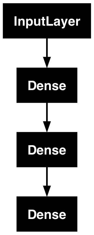
请考虑以下模型：

(input: 784-dimensional vectors) ↧ [Dense (64 units, relu activation)] ↧ [Dense (64 units, relu activation)] ↧ [Dense (10 units, softmax activation)] ↧ (output: logits of a probability distribution over 10 classes)

这是一个包含三层的基本图形。要使用函数式 API 构建此模型，请先创建一个 input 节点：

inputs = keras.Input(shape=(784,))

数据的形状设置为 784 维向量。由于仅指定了每个样本的形状，因此始终省略批量大小。

例如，如果您有一个形状为，您将使用：(32, 32, 3)

# Just for demonstration purposes.
img_inputs = keras.Input(shape=(32, 32, 3))

返回的包含有关形状和馈送到模型的输入数据的信息。这是形状：inputsdtype

inputs.shape

(None, 784)

下面是 dtype：

inputs.dtype

'float32'

您可以通过在此对象上调用一个层，在层图中创建新节点：inputs

dense = layers.Dense(64, activation="relu")
x = dense(inputs)

“图层调用”作类似于从 “inputs” 向此图层绘制箭头您创建的。您将输入“传递”到层，并获取作为输出。densex

让我们在层图中再添加几个层：

x = layers.Dense(64, activation="relu")(x)
outputs = layers.Dense(10)(x)

此时，您可以通过指定其输入和输出来创建在 Layers 的图形中：Model

model = keras.Model(inputs=inputs, outputs=outputs, name="mnist_model")

让我们看看模型摘要是什么样的：

model.summary()

Model: "mnist_model"

┏━━━━━━━━━━━━━━━━━━━━━━━━━━━━━━━━━┳━━━━━━━━━━━━━━━━━━━━━━━━┳━━━━━━━━━━━━━━━┓
┃ Layer (type)                    ┃ Output Shape           ┃       Param # ┃
┡━━━━━━━━━━━━━━━━━━━━━━━━━━━━━━━━━╇━━━━━━━━━━━━━━━━━━━━━━━━╇━━━━━━━━━━━━━━━┩
│ input_layer (InputLayer)        │ (None, 784)            │             0 │
├─────────────────────────────────┼────────────────────────┼───────────────┤
│ dense (Dense)                   │ (None, 64)             │        50,240 │
├─────────────────────────────────┼────────────────────────┼───────────────┤
│ dense_1 (Dense)                 │ (None, 64)             │         4,160 │
├─────────────────────────────────┼────────────────────────┼───────────────┤
│ dense_2 (Dense)                 │ (None, 10)             │           650 │
└─────────────────────────────────┴────────────────────────┴───────────────┘

 Total params: 55,050 (215.04 KB)

 Trainable params: 55,050 (215.04 KB)

 Non-trainable params: 0 (0.00 B)

您还可以将模型绘制为图形：

keras.utils.plot_model(model, "my_first_model.png")

PNG 格式

并且，还可以选择显示每个图层的输入和输出形状在绘制的图形中：

keras.utils.plot_model(model, "my_first_model_with_shape_info.png", show_shapes=True)

PNG 格式

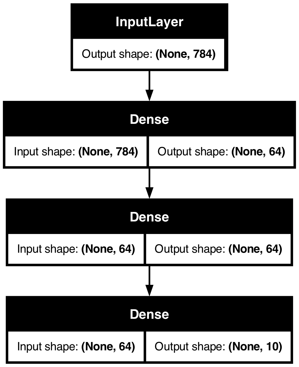
此图和代码几乎相同。在代码版本中，连接箭头将替换为 call作。

“层图”是深度学习模型的直观心理图像，而函数式 API 是一种创建与此密切相关的模型的方法。

训练、评估和推理

模型的训练、评估和推理的工作方式完全相同使用函数式 API 构建，与模型一样。Sequential

该类提供了一个内置的训练循环（方法）以及一个内置的 Evaluation Loop （方法）。注意您可以轻松自定义这些循环以实施您自己的训练程序。另请参阅有关自定义中发生的事情的指南：Modelfit()evaluate()fit()

使用 TensorFlow 编写自定义训练步骤
使用 JAX 编写自定义训练步骤
使用 PyTorch 编写自定义训练步骤

在这里，加载 MNIST 图像数据，将其修整为向量，在数据上拟合模型（同时监控验证拆分的性能），然后根据测试数据评估模型：

(x_train, y_train), (x_test, y_test) = keras.datasets.mnist.load_data()

x_train = x_train.reshape(60000, 784).astype("float32") / 255
x_test = x_test.reshape(10000, 784).astype("float32") / 255

model.compile(
    loss=keras.losses.SparseCategoricalCrossentropy(from_logits=True),
    optimizer=keras.optimizers.RMSprop(),
    metrics=["accuracy"],
)

history = model.fit(x_train, y_train, batch_size=64, epochs=2, validation_split=0.2)

test_scores = model.evaluate(x_test, y_test, verbose=2)
print("Test loss:", test_scores[0])
print("Test accuracy:", test_scores[1])

Epoch 1/2 750/750 ━━━━━━━━━━━━━━━━━━━━ 1s 863us/step - accuracy: 0.8425 - loss: 0.5733 - val_accuracy: 0.9496 - val_loss: 0.1711 Epoch 2/2 750/750 ━━━━━━━━━━━━━━━━━━━━ 1s 859us/step - accuracy: 0.9509 - loss: 0.1641 - val_accuracy: 0.9578 - val_loss: 0.1396 313/313 - 0s - 341us/step - accuracy: 0.9613 - loss: 0.1288 Test loss: 0.12876172363758087 Test accuracy: 0.9613000154495239

如需进一步阅读，请参阅培训和评估指南。

保存和序列化

保存模型和序列化的工作方式与使用函数式 API。标准方式保存功能模型就是调用将整个模型保存为单个文件。您可以稍后重新创建相同的模型从此文件中，即使构建模型的代码不再可用。Sequentialmodel.save()

此保存的文件包括： - 模型架构 - 模型权重值（在训练期间学习） - 模型训练配置（如果有）（传递给） - Optimizer 及其状态（如果有）（从上次中断的地方重新开始训练）compile()

model.save("my_model.keras")
del model
# Recreate the exact same model purely from the file:
model = keras.models.load_model("my_model.keras")

有关详细信息，请阅读模型序列化和保存指南。

使用相同的层图定义多个模型

在函数式 API 中，通过指定模型的输入来创建模型和层图中的输出。这意味着单个图层图可用于生成多个模型。

在下面的示例中，您使用相同的层堆栈来实例化两个模型：一个将图像输入转换为 16 维向量的模型，以及用于训练的端到端模型。encoderautoencoder

encoder_input = keras.Input(shape=(28, 28, 1), name="img")
x = layers.Conv2D(16, 3, activation="relu")(encoder_input)
x = layers.Conv2D(32, 3, activation="relu")(x)
x = layers.MaxPooling2D(3)(x)
x = layers.Conv2D(32, 3, activation="relu")(x)
x = layers.Conv2D(16, 3, activation="relu")(x)
encoder_output = layers.GlobalMaxPooling2D()(x)

encoder = keras.Model(encoder_input, encoder_output, name="encoder")
encoder.summary()

x = layers.Reshape((4, 4, 1))(encoder_output)
x = layers.Conv2DTranspose(16, 3, activation="relu")(x)
x = layers.Conv2DTranspose(32, 3, activation="relu")(x)
x = layers.UpSampling2D(3)(x)
x = layers.Conv2DTranspose(16, 3, activation="relu")(x)
decoder_output = layers.Conv2DTranspose(1, 3, activation="relu")(x)

autoencoder = keras.Model(encoder_input, decoder_output, name="autoencoder")
autoencoder.summary()

Model: "encoder"

┏━━━━━━━━━━━━━━━━━━━━━━━━━━━━━━━━━┳━━━━━━━━━━━━━━━━━━━━━━━━┳━━━━━━━━━━━━━━━┓
┃ Layer (type)                    ┃ Output Shape           ┃       Param # ┃
┡━━━━━━━━━━━━━━━━━━━━━━━━━━━━━━━━━╇━━━━━━━━━━━━━━━━━━━━━━━━╇━━━━━━━━━━━━━━━┩
│ img (InputLayer)                │ (None, 28, 28, 1)      │             0 │
├─────────────────────────────────┼────────────────────────┼───────────────┤
│ conv2d (Conv2D)                 │ (None, 26, 26, 16)     │           160 │
├─────────────────────────────────┼────────────────────────┼───────────────┤
│ conv2d_1 (Conv2D)               │ (None, 24, 24, 32)     │         4,640 │
├─────────────────────────────────┼────────────────────────┼───────────────┤
│ max_pooling2d (MaxPooling2D)    │ (None, 8, 8, 32)       │             0 │
├─────────────────────────────────┼────────────────────────┼───────────────┤
│ conv2d_2 (Conv2D)               │ (None, 6, 6, 32)       │         9,248 │
├─────────────────────────────────┼────────────────────────┼───────────────┤
│ conv2d_3 (Conv2D)               │ (None, 4, 4, 16)       │         4,624 │
├─────────────────────────────────┼────────────────────────┼───────────────┤
│ global_max_pooling2d            │ (None, 16)             │             0 │
│ (GlobalMaxPooling2D)            │                        │               │
└─────────────────────────────────┴────────────────────────┴───────────────┘

 Total params: 18,672 (72.94 KB)

 Trainable params: 18,672 (72.94 KB)

 Non-trainable params: 0 (0.00 B)

Model: "autoencoder"

┏━━━━━━━━━━━━━━━━━━━━━━━━━━━━━━━━━┳━━━━━━━━━━━━━━━━━━━━━━━━┳━━━━━━━━━━━━━━━┓
┃ Layer (type)                    ┃ Output Shape           ┃       Param # ┃
┡━━━━━━━━━━━━━━━━━━━━━━━━━━━━━━━━━╇━━━━━━━━━━━━━━━━━━━━━━━━╇━━━━━━━━━━━━━━━┩
│ img (InputLayer)                │ (None, 28, 28, 1)      │             0 │
├─────────────────────────────────┼────────────────────────┼───────────────┤
│ conv2d (Conv2D)                 │ (None, 26, 26, 16)     │           160 │
├─────────────────────────────────┼────────────────────────┼───────────────┤
│ conv2d_1 (Conv2D)               │ (None, 24, 24, 32)     │         4,640 │
├─────────────────────────────────┼────────────────────────┼───────────────┤
│ max_pooling2d (MaxPooling2D)    │ (None, 8, 8, 32)       │             0 │
├─────────────────────────────────┼────────────────────────┼───────────────┤
│ conv2d_2 (Conv2D)               │ (None, 6, 6, 32)       │         9,248 │
├─────────────────────────────────┼────────────────────────┼───────────────┤
│ conv2d_3 (Conv2D)               │ (None, 4, 4, 16)       │         4,624 │
├─────────────────────────────────┼────────────────────────┼───────────────┤
│ global_max_pooling2d            │ (None, 16)             │             0 │
│ (GlobalMaxPooling2D)            │                        │               │
├─────────────────────────────────┼────────────────────────┼───────────────┤
│ reshape (Reshape)               │ (None, 4, 4, 1)        │             0 │
├─────────────────────────────────┼────────────────────────┼───────────────┤
│ conv2d_transpose                │ (None, 6, 6, 16)       │           160 │
│ (Conv2DTranspose)               │                        │               │
├─────────────────────────────────┼────────────────────────┼───────────────┤
│ conv2d_transpose_1              │ (None, 8, 8, 32)       │         4,640 │
│ (Conv2DTranspose)               │                        │               │
├─────────────────────────────────┼────────────────────────┼───────────────┤
│ up_sampling2d (UpSampling2D)    │ (None, 24, 24, 32)     │             0 │
├─────────────────────────────────┼────────────────────────┼───────────────┤
│ conv2d_transpose_2              │ (None, 26, 26, 16)     │         4,624 │
│ (Conv2DTranspose)               │                        │               │
├─────────────────────────────────┼────────────────────────┼───────────────┤
│ conv2d_transpose_3              │ (None, 28, 28, 1)      │           145 │
│ (Conv2DTranspose)               │                        │               │
└─────────────────────────────────┴────────────────────────┴───────────────┘

 Total params: 28,241 (110.32 KB)

 Trainable params: 28,241 (110.32 KB)

 Non-trainable params: 0 (0.00 B)

在这里，解码架构是严格对称的添加到编码体系结构中，因此输出形状与输入 shape .(28, 28, 1)

图层的反面是图层，图层的反面是图层。Conv2DConv2DTransposeMaxPooling2DUpSampling2D

所有模型都是可调用的，就像 layers 一样

您可以通过在或上调用任何模型来将任何模型视为一个层在另一个层的输出上。通过调用模型，您不仅仅是在重用模型的架构，您也在重用其权重。Input

为了实际查看这一点，以下是对自动编码器示例的不同看法：创建一个编码器模型、一个解码器模型，并将它们链接在两个调用中要获取 autoencoder 模型，请执行以下作：

encoder_input = keras.Input(shape=(28, 28, 1), name="original_img")
x = layers.Conv2D(16, 3, activation="relu")(encoder_input)
x = layers.Conv2D(32, 3, activation="relu")(x)
x = layers.MaxPooling2D(3)(x)
x = layers.Conv2D(32, 3, activation="relu")(x)
x = layers.Conv2D(16, 3, activation="relu")(x)
encoder_output = layers.GlobalMaxPooling2D()(x)

encoder = keras.Model(encoder_input, encoder_output, name="encoder")
encoder.summary()

decoder_input = keras.Input(shape=(16,), name="encoded_img")
x = layers.Reshape((4, 4, 1))(decoder_input)
x = layers.Conv2DTranspose(16, 3, activation="relu")(x)
x = layers.Conv2DTranspose(32, 3, activation="relu")(x)
x = layers.UpSampling2D(3)(x)
x = layers.Conv2DTranspose(16, 3, activation="relu")(x)
decoder_output = layers.Conv2DTranspose(1, 3, activation="relu")(x)

decoder = keras.Model(decoder_input, decoder_output, name="decoder")
decoder.summary()

autoencoder_input = keras.Input(shape=(28, 28, 1), name="img")
encoded_img = encoder(autoencoder_input)
decoded_img = decoder(encoded_img)
autoencoder = keras.Model(autoencoder_input, decoded_img, name="autoencoder")
autoencoder.summary()

Model: "encoder"

┏━━━━━━━━━━━━━━━━━━━━━━━━━━━━━━━━━┳━━━━━━━━━━━━━━━━━━━━━━━━┳━━━━━━━━━━━━━━━┓
┃ Layer (type)                    ┃ Output Shape           ┃       Param # ┃
┡━━━━━━━━━━━━━━━━━━━━━━━━━━━━━━━━━╇━━━━━━━━━━━━━━━━━━━━━━━━╇━━━━━━━━━━━━━━━┩
│ original_img (InputLayer)       │ (None, 28, 28, 1)      │             0 │
├─────────────────────────────────┼────────────────────────┼───────────────┤
│ conv2d_4 (Conv2D)               │ (None, 26, 26, 16)     │           160 │
├─────────────────────────────────┼────────────────────────┼───────────────┤
│ conv2d_5 (Conv2D)               │ (None, 24, 24, 32)     │         4,640 │
├─────────────────────────────────┼────────────────────────┼───────────────┤
│ max_pooling2d_1 (MaxPooling2D)  │ (None, 8, 8, 32)       │             0 │
├─────────────────────────────────┼────────────────────────┼───────────────┤
│ conv2d_6 (Conv2D)               │ (None, 6, 6, 32)       │         9,248 │
├─────────────────────────────────┼────────────────────────┼───────────────┤
│ conv2d_7 (Conv2D)               │ (None, 4, 4, 16)       │         4,624 │
├─────────────────────────────────┼────────────────────────┼───────────────┤
│ global_max_pooling2d_1          │ (None, 16)             │             0 │
│ (GlobalMaxPooling2D)            │                        │               │
└─────────────────────────────────┴────────────────────────┴───────────────┘

 Total params: 18,672 (72.94 KB)

 Trainable params: 18,672 (72.94 KB)

 Non-trainable params: 0 (0.00 B)

Model: "decoder"

┏━━━━━━━━━━━━━━━━━━━━━━━━━━━━━━━━━┳━━━━━━━━━━━━━━━━━━━━━━━━┳━━━━━━━━━━━━━━━┓
┃ Layer (type)                    ┃ Output Shape           ┃       Param # ┃
┡━━━━━━━━━━━━━━━━━━━━━━━━━━━━━━━━━╇━━━━━━━━━━━━━━━━━━━━━━━━╇━━━━━━━━━━━━━━━┩
│ encoded_img (InputLayer)        │ (None, 16)             │             0 │
├─────────────────────────────────┼────────────────────────┼───────────────┤
│ reshape_1 (Reshape)             │ (None, 4, 4, 1)        │             0 │
├─────────────────────────────────┼────────────────────────┼───────────────┤
│ conv2d_transpose_4              │ (None, 6, 6, 16)       │           160 │
│ (Conv2DTranspose)               │                        │               │
├─────────────────────────────────┼────────────────────────┼───────────────┤
│ conv2d_transpose_5              │ (None, 8, 8, 32)       │         4,640 │
│ (Conv2DTranspose)               │                        │               │
├─────────────────────────────────┼────────────────────────┼───────────────┤
│ up_sampling2d_1 (UpSampling2D)  │ (None, 24, 24, 32)     │             0 │
├─────────────────────────────────┼────────────────────────┼───────────────┤
│ conv2d_transpose_6              │ (None, 26, 26, 16)     │         4,624 │
│ (Conv2DTranspose)               │                        │               │
├─────────────────────────────────┼────────────────────────┼───────────────┤
│ conv2d_transpose_7              │ (None, 28, 28, 1)      │           145 │
│ (Conv2DTranspose)               │                        │               │
└─────────────────────────────────┴────────────────────────┴───────────────┘

 Total params: 9,569 (37.38 KB)

 Trainable params: 9,569 (37.38 KB)

 Non-trainable params: 0 (0.00 B)

Model: "autoencoder"

┏━━━━━━━━━━━━━━━━━━━━━━━━━━━━━━━━━┳━━━━━━━━━━━━━━━━━━━━━━━━┳━━━━━━━━━━━━━━━┓
┃ Layer (type)                    ┃ Output Shape           ┃       Param # ┃
┡━━━━━━━━━━━━━━━━━━━━━━━━━━━━━━━━━╇━━━━━━━━━━━━━━━━━━━━━━━━╇━━━━━━━━━━━━━━━┩
│ img (InputLayer)                │ (None, 28, 28, 1)      │             0 │
├─────────────────────────────────┼────────────────────────┼───────────────┤
│ encoder (Functional)            │ (None, 16)             │        18,672 │
├─────────────────────────────────┼────────────────────────┼───────────────┤
│ decoder (Functional)            │ (None, 28, 28, 1)      │         9,569 │
└─────────────────────────────────┴────────────────────────┴───────────────┘

 Total params: 28,241 (110.32 KB)

 Trainable params: 28,241 (110.32 KB)

 Non-trainable params: 0 (0.00 B)

如您所见，模型可以嵌套：一个模型可以包含子模型（因为模型就像一个层）。模型嵌套的一个常见用例是集成。例如，下面介绍如何将一组模型集成为单个模型这平均了他们的预测：

def get_model():
    inputs = keras.Input(shape=(128,))
    outputs = layers.Dense(1)(inputs)
    return keras.Model(inputs, outputs)


model1 = get_model()
model2 = get_model()
model3 = get_model()

inputs = keras.Input(shape=(128,))
y1 = model1(inputs)
y2 = model2(inputs)
y3 = model3(inputs)
outputs = layers.average([y1, y2, y3])
ensemble_model = keras.Model(inputs=inputs, outputs=outputs)

作复杂的图形拓扑

具有多个输入和输出的模型

函数式 API 可以轻松作多个输入和输出。这无法使用 API 处理。Sequential

例如，如果您正在构建一个系统，用于按以下条件对客户问题工单进行排名 priority 并将它们路由到正确的部门，然后，模型将有三个输入：

工单的标题（文本输入），
工单的文本正文（文本输入），以及
用户添加的任何标记（分类输入）

此模型将有两个输出：

介于 0 和 1 之间的优先级分数（标量 sigmoid 输出），以及
应处理工单的部门（SoftMax 输出在一组部门上）。

您可以使用函数式 API 通过几行代码构建此模型：

num_tags = 12  # Number of unique issue tags
num_words = 10000  # Size of vocabulary obtained when preprocessing text data
num_departments = 4  # Number of departments for predictions

title_input = keras.Input(
    shape=(None,), name="title"
)  # Variable-length sequence of ints
body_input = keras.Input(shape=(None,), name="body")  # Variable-length sequence of ints
tags_input = keras.Input(
    shape=(num_tags,), name="tags"
)  # Binary vectors of size `num_tags`

# Embed each word in the title into a 64-dimensional vector
title_features = layers.Embedding(num_words, 64)(title_input)
# Embed each word in the text into a 64-dimensional vector
body_features = layers.Embedding(num_words, 64)(body_input)

# Reduce sequence of embedded words in the title into a single 128-dimensional vector
title_features = layers.LSTM(128)(title_features)
# Reduce sequence of embedded words in the body into a single 32-dimensional vector
body_features = layers.LSTM(32)(body_features)

# Merge all available features into a single large vector via concatenation
x = layers.concatenate([title_features, body_features, tags_input])

# Stick a logistic regression for priority prediction on top of the features
priority_pred = layers.Dense(1, name="priority")(x)
# Stick a department classifier on top of the features
department_pred = layers.Dense(num_departments, name="department")(x)

# Instantiate an end-to-end model predicting both priority and department
model = keras.Model(
    inputs=[title_input, body_input, tags_input],
    outputs={"priority": priority_pred, "department": department_pred},
)

现在绘制模型：

keras.utils.plot_model(model, "multi_input_and_output_model.png", show_shapes=True)

PNG 格式

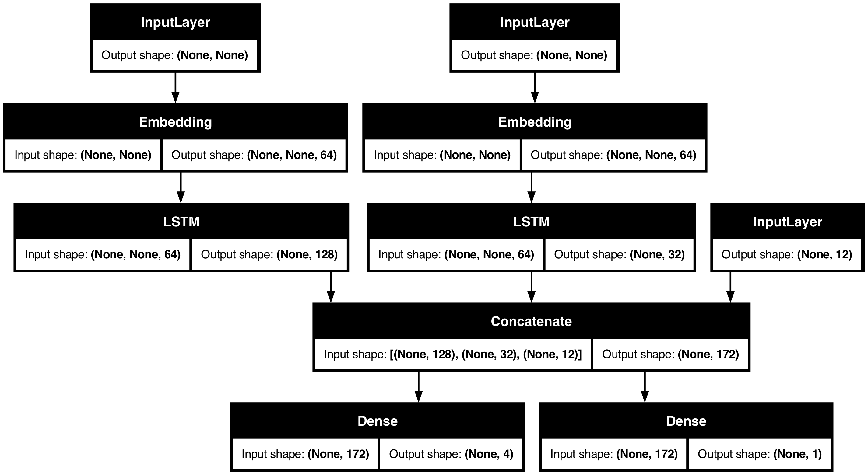
编译此模型时，您可以为每个输出分配不同的损失。您甚至可以为每个损失分配不同的权重 - 进行调制他们对总训练损失的贡献。

model.compile(
    optimizer=keras.optimizers.RMSprop(1e-3),
    loss=[
        keras.losses.BinaryCrossentropy(from_logits=True),
        keras.losses.CategoricalCrossentropy(from_logits=True),
    ],
    loss_weights=[1.0, 0.2],
)

由于输出图层具有不同的名称，因此您还可以指定具有相应图层名称的 losses 和 loss weights：

model.compile(
    optimizer=keras.optimizers.RMSprop(1e-3),
    loss={
        "priority": keras.losses.BinaryCrossentropy(from_logits=True),
        "department": keras.losses.CategoricalCrossentropy(from_logits=True),
    },
    loss_weights={"priority": 1.0, "department": 0.2},
)

通过传递输入和目标的 NumPy 数组列表来训练模型：

# Dummy input data
title_data = np.random.randint(num_words, size=(1280, 12))
body_data = np.random.randint(num_words, size=(1280, 100))
tags_data = np.random.randint(2, size=(1280, num_tags)).astype("float32")

# Dummy target data
priority_targets = np.random.random(size=(1280, 1))
dept_targets = np.random.randint(2, size=(1280, num_departments))

model.fit(
    {"title": title_data, "body": body_data, "tags": tags_data},
    {"priority": priority_targets, "department": dept_targets},
    epochs=2,
    batch_size=32,
)

Epoch 1/2 40/40 ━━━━━━━━━━━━━━━━━━━━ 3s 57ms/step - loss: 1108.3792 Epoch 2/2 40/40 ━━━━━━━━━━━━━━━━━━━━ 2s 54ms/step - loss: 621.3049 <keras.src.callbacks.history.History at 0x34afc3d90>

当对对象调用 fit 时，它应该产生一个像这样的列表元组或像 .Dataset([title_data, body_data, tags_data], [priority_targets, dept_targets])({'title': title_data, 'body': body_data, 'tags': tags_data}, {'priority': priority_targets, 'department': dept_targets})

有关更详细的说明，请参阅训练和评估指南.

玩具 ResNet 模型

除了具有多个输入和输出的模型外，函数式 API 使作非线性连接变得容易拓扑 – 这些是具有未按顺序连接的层的模型， API 无法处理。Sequential

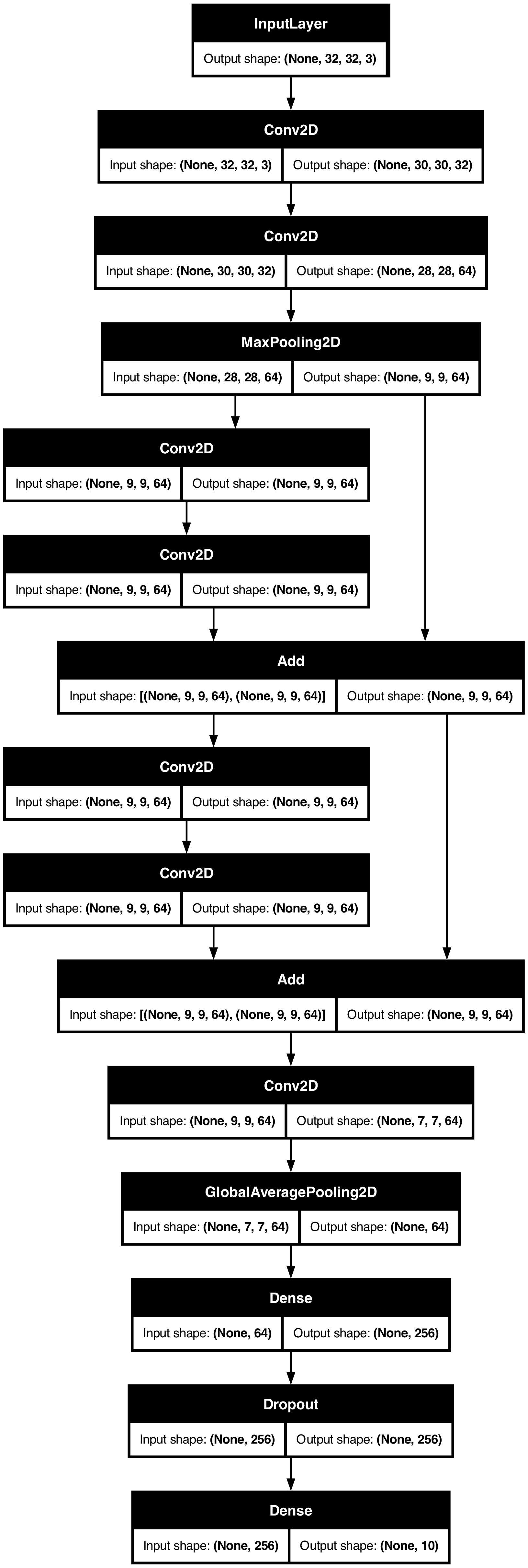
这种情况的一个常见用例是残差连接。让我们为 CIFAR10 构建一个玩具 ResNet 模型来演示这一点：

inputs = keras.Input(shape=(32, 32, 3), name="img")
x = layers.Conv2D(32, 3, activation="relu")(inputs)
x = layers.Conv2D(64, 3, activation="relu")(x)
block_1_output = layers.MaxPooling2D(3)(x)

x = layers.Conv2D(64, 3, activation="relu", padding="same")(block_1_output)
x = layers.Conv2D(64, 3, activation="relu", padding="same")(x)
block_2_output = layers.add([x, block_1_output])

x = layers.Conv2D(64, 3, activation="relu", padding="same")(block_2_output)
x = layers.Conv2D(64, 3, activation="relu", padding="same")(x)
block_3_output = layers.add([x, block_2_output])

x = layers.Conv2D(64, 3, activation="relu")(block_3_output)
x = layers.GlobalAveragePooling2D()(x)
x = layers.Dense(256, activation="relu")(x)
x = layers.Dropout(0.5)(x)
outputs = layers.Dense(10)(x)

model = keras.Model(inputs, outputs, name="toy_resnet")
model.summary()

Model: "toy_resnet"

┏━━━━━━━━━━━━━━━━━━━━━┳━━━━━━━━━━━━━━━━━━━┳━━━━━━━━━━━━┳━━━━━━━━━━━━━━━━━━━┓
┃ Layer (type)        ┃ Output Shape      ┃    Param # ┃ Connected to      ┃
┡━━━━━━━━━━━━━━━━━━━━━╇━━━━━━━━━━━━━━━━━━━╇━━━━━━━━━━━━╇━━━━━━━━━━━━━━━━━━━┩
│ img (InputLayer)    │ (None, 32, 32, 3) │          0 │ -                 │
├─────────────────────┼───────────────────┼────────────┼───────────────────┤
│ conv2d_8 (Conv2D)   │ (None, 30, 30,    │        896 │ img[0][0]         │
│                     │ 32)               │            │                   │
├─────────────────────┼───────────────────┼────────────┼───────────────────┤
│ conv2d_9 (Conv2D)   │ (None, 28, 28,    │     18,496 │ conv2d_8[0][0]    │
│                     │ 64)               │            │                   │
├─────────────────────┼───────────────────┼────────────┼───────────────────┤
│ max_pooling2d_2     │ (None, 9, 9, 64)  │          0 │ conv2d_9[0][0]    │
│ (MaxPooling2D)      │                   │            │                   │
├─────────────────────┼───────────────────┼────────────┼───────────────────┤
│ conv2d_10 (Conv2D)  │ (None, 9, 9, 64)  │     36,928 │ max_pooling2d_2[… │
├─────────────────────┼───────────────────┼────────────┼───────────────────┤
│ conv2d_11 (Conv2D)  │ (None, 9, 9, 64)  │     36,928 │ conv2d_10[0][0]   │
├─────────────────────┼───────────────────┼────────────┼───────────────────┤
│ add (Add)           │ (None, 9, 9, 64)  │          0 │ conv2d_11[0][0],  │
│                     │                   │            │ max_pooling2d_2[… │
├─────────────────────┼───────────────────┼────────────┼───────────────────┤
│ conv2d_12 (Conv2D)  │ (None, 9, 9, 64)  │     36,928 │ add[0][0]         │
├─────────────────────┼───────────────────┼────────────┼───────────────────┤
│ conv2d_13 (Conv2D)  │ (None, 9, 9, 64)  │     36,928 │ conv2d_12[0][0]   │
├─────────────────────┼───────────────────┼────────────┼───────────────────┤
│ add_1 (Add)         │ (None, 9, 9, 64)  │          0 │ conv2d_13[0][0],  │
│                     │                   │            │ add[0][0]         │
├─────────────────────┼───────────────────┼────────────┼───────────────────┤
│ conv2d_14 (Conv2D)  │ (None, 7, 7, 64)  │     36,928 │ add_1[0][0]       │
├─────────────────────┼───────────────────┼────────────┼───────────────────┤
│ global_average_poo… │ (None, 64)        │          0 │ conv2d_14[0][0]   │
│ (GlobalAveragePool… │                   │            │                   │
├─────────────────────┼───────────────────┼────────────┼───────────────────┤
│ dense_6 (Dense)     │ (None, 256)       │     16,640 │ global_average_p… │
├─────────────────────┼───────────────────┼────────────┼───────────────────┤
│ dropout (Dropout)   │ (None, 256)       │          0 │ dense_6[0][0]     │
├─────────────────────┼───────────────────┼────────────┼───────────────────┤
│ dense_7 (Dense)     │ (None, 10)        │      2,570 │ dropout[0][0]     │
└─────────────────────┴───────────────────┴────────────┴───────────────────┘

 Total params: 223,242 (872.04 KB)

 Trainable params: 223,242 (872.04 KB)

 Non-trainable params: 0 (0.00 B)

绘制模型：

keras.utils.plot_model(model, "mini_resnet.png", show_shapes=True)

PNG 格式

现在训练模型：

(x_train, y_train), (x_test, y_test) = keras.datasets.cifar10.load_data()

x_train = x_train.astype("float32") / 255.0
x_test = x_test.astype("float32") / 255.0
y_train = keras.utils.to_categorical(y_train, 10)
y_test = keras.utils.to_categorical(y_test, 10)

model.compile(
    optimizer=keras.optimizers.RMSprop(1e-3),
    loss=keras.losses.CategoricalCrossentropy(from_logits=True),
    metrics=["acc"],
)
# We restrict the data to the first 1000 samples so as to limit execution time
# on Colab. Try to train on the entire dataset until convergence!
model.fit(
    x_train[:1000],
    y_train[:1000],
    batch_size=64,
    epochs=1,
    validation_split=0.2,
)

 13/13 ━━━━━━━━━━━━━━━━━━━━ 1s 60ms/step - acc: 0.1096 - loss: 2.3053 - val_acc: 0.1150 - val_loss: 2.2973 <keras.src.callbacks.history.History at 0x1758bed40>

共享层

函数式 API 的另一个好用途是使用共享层的模型。共享层是在同一模型中多次重复使用的层实例 – 他们学习对应于层图中的多条路径的特征。

共享层通常用于对来自相似空间的输入进行编码（例如，具有相似词汇的两段不同的文本）。它们支持在这些不同的输入之间共享信息。它们使得使用更少的数据训练这样的模型成为可能。如果在其中一个输入中看到给定的单词，则这将有利于处理通过共享层的所有输入。

要在功能 API 中共享层，请多次调用同一层实例。例如，下面是一个在两个不同的文本输入之间共享的图层：Embedding

# Embedding for 1000 unique words mapped to 128-dimensional vectors
shared_embedding = layers.Embedding(1000, 128)

# Variable-length sequence of integers
text_input_a = keras.Input(shape=(None,), dtype="int32")

# Variable-length sequence of integers
text_input_b = keras.Input(shape=(None,), dtype="int32")

# Reuse the same layer to encode both inputs
encoded_input_a = shared_embedding(text_input_a)
encoded_input_b = shared_embedding(text_input_b)

提取和重用图层图中的节点

因为您正在处理的图层图是静态数据结构，可以访问和检查它。这就是您能够绘制的方式功能模型作为图像。

这也意味着您可以访问中间层的激活（图中的 “nodes”）并在其他位置重用它们 – 这对于特征提取之类的事情非常有用。

让我们看一个例子。这是一个在 ImageNet 上预训练权重的 VGG19 模型：

vgg19 = keras.applications.VGG19()

这些是模型的中间激活，通过查询 Graph 数据结构获得：

features_list = [layer.output for layer in vgg19.layers]

使用这些特征来创建新的特征提取模型，该模型返回中间层 activations 的值：

feat_extraction_model = keras.Model(inputs=vgg19.input, outputs=features_list)

img = np.random.random((1, 224, 224, 3)).astype("float32")
extracted_features = feat_extraction_model(img)

这对于神经样式迁移、除其他外。

使用自定义层扩展 API

keras包括各种内置图层，例如：

卷积层：、、、Conv1DConv2DConv3DConv2DTranspose
池化层：、MaxPooling1DMaxPooling2DMaxPooling3DAveragePooling1D
RNN 层：、、GRULSTMConvLSTM2D
BatchNormalization等。DropoutEmbedding

但是，如果你没有找到你需要的东西，很容易通过创建您自己的图层。所有层都子类化了类并实现：Layer

call方法，指定层完成的计算。
build方法创建图层的权重（这只是一种样式约定，因为您也可以在中创建权重）。__init__

要了解有关从头开始创建图层的更多信息，请阅读自定义图层和模型指南。

以下是 keras.layers.Dense 的基本实现：

class CustomDense(layers.Layer):
    def __init__(self, units=32):
        super().__init__()
        self.units = units

    def build(self, input_shape):
        self.w = self.add_weight(
            shape=(input_shape[-1], self.units),
            initializer="random_normal",
            trainable=True,
        )
        self.b = self.add_weight(
            shape=(self.units,), initializer="random_normal", trainable=True
        )

    def call(self, inputs):
        return ops.matmul(inputs, self.w) + self.b


inputs = keras.Input((4,))
outputs = CustomDense(10)(inputs)

model = keras.Model(inputs, outputs)

对于自定义层中的序列化支持，请定义一个返回层实例的构造函数参数的方法：get_config()

class CustomDense(layers.Layer):
    def __init__(self, units=32):
        super().__init__()
        self.units = units

    def build(self, input_shape):
        self.w = self.add_weight(
            shape=(input_shape[-1], self.units),
            initializer="random_normal",
            trainable=True,
        )
        self.b = self.add_weight(
            shape=(self.units,), initializer="random_normal", trainable=True
        )

    def call(self, inputs):
        return ops.matmul(inputs, self.w) + self.b

    def get_config(self):
        return {"units": self.units}


inputs = keras.Input((4,))
outputs = CustomDense(10)(inputs)

model = keras.Model(inputs, outputs)
config = model.get_config()

new_model = keras.Model.from_config(config, custom_objects={"CustomDense": CustomDense})

（可选）实现使用的类方法在给定其 config 字典的情况下重新创建 Layer 实例时。的默认实现是：from_config(cls, config)from_config

def from_config(cls, config):
  return cls(**config)

何时使用功能式 API

如果您使用 Keras 函数式 API 创建新模型，或者只是直接子类化类？一般来说，函数式 API 更高层次、更简单、更安全，并拥有多项子类化模型不支持的功能。Model

但是，模型子类化在构建模型时提供了更大的灵活性不容易表示为层的有向无环图。例如，您无法使用函数式 API 实现 Tree-RNN 并且必须直接 subclass。Model

要深入了解函数式 API 和 model 子类化，请参阅什么是 TensorFlow 2.0 中的符号 API 和命令式 API？。

功能性 API 优势：

以下属性也适用于 Sequential 模型（也是数据结构），但对于子类化模型则不然（这是 Python 字节码，而不是数据结构）。

不那么冗长

没有，没有，等等。super().__init__(...)def call(self, ...):

比较：

inputs = keras.Input(shape=(32,))
x = layers.Dense(64, activation='relu')(inputs)
outputs = layers.Dense(10)(x)
mlp = keras.Model(inputs, outputs)

使用子类化版本：

class MLP(keras.Model):

  def __init__(self, **kwargs):
    super().__init__(**kwargs)
    self.dense_1 = layers.Dense(64, activation='relu')
    self.dense_2 = layers.Dense(10)

  def call(self, inputs):
    x = self.dense_1(inputs)
    return self.dense_2(x)

# Instantiate the model.
mlp = MLP()
# Necessary to create the model's state.
# The model doesn't have a state until it's called at least once.
_ = mlp(ops.zeros((1, 32)))

在定义其连接图时进行模型验证

在函数式 API 中，创建输入规范（shape 和 dtype）提前（使用）。每次调用一个层时，该层检查传递给它的规范是否与其假设匹配。如果没有，它将引发一个有用的错误消息。Input

这保证了您可以使用函数式 API 构建的任何模型都将运行。所有调试 – 除了与收敛相关的调试 – 在模型构造期间静态发生，而不是在执行时发生。这类似于编译器中的类型检查。

功能模型是可绘制和可检查的

您可以将模型绘制为图形，并且可以轻松访问中间节点在此图中。例如，要提取和重用中间层（如前面的示例所示）：

features_list = [layer.output for layer in vgg19.layers]
feat_extraction_model = keras.Model(inputs=vgg19.input, outputs=features_list)

功能模型可以序列化或克隆

因为函数式模型是一个数据结构，而不是一段代码，它是可安全序列化的，并且可以保存为单个文件，允许您重新创建完全相同的模型无法访问任何原始代码。请参阅序列化和保存指南。

要序列化子类化模型，实现者必须以在模型级别指定 AND 方法。get_config()from_config()

功能性 API 弱点：

它不支持动态架构

函数式 API 将模型视为层的 DAG。大多数深度学习架构都是如此，但并非全部都是如此，例如，递归网络或树 RNN 不遵循此假设，也不能在函数式 API 中实现。

混合搭配 API 样式

在函数式 API 或 Model 子类化之间进行选择不是 Binary 决策，该决策将您限制在一类模型中。 API 中的所有模型都可以相互交互，无论它们是模型、函数模型还是编写的子类化模型白手起家。kerasSequential

您始终可以使用函数模型或模型作为子类化模型或层的一部分：Sequential

units = 32
timesteps = 10
input_dim = 5

# Define a Functional model
inputs = keras.Input((None, units))
x = layers.GlobalAveragePooling1D()(inputs)
outputs = layers.Dense(1)(x)
model = keras.Model(inputs, outputs)


class CustomRNN(layers.Layer):
    def __init__(self):
        super().__init__()
        self.units = units
        self.projection_1 = layers.Dense(units=units, activation="tanh")
        self.projection_2 = layers.Dense(units=units, activation="tanh")
        # Our previously-defined Functional model
        self.classifier = model

    def call(self, inputs):
        outputs = []
        state = ops.zeros(shape=(inputs.shape[0], self.units))
        for t in range(inputs.shape[1]):
            x = inputs[:, t, :]
            h = self.projection_1(x)
            y = h + self.projection_2(state)
            state = y
            outputs.append(y)
        features = ops.stack(outputs, axis=1)
        print(features.shape)
        return self.classifier(features)


rnn_model = CustomRNN()
_ = rnn_model(ops.zeros((1, timesteps, input_dim)))

(1, 10, 32) (1, 10, 32)

您可以在函数式 API 中使用任何子类化层或模型只要它实现遵循以下模式之一的方法：call

call(self, inputs, **kwargs)– 其中是张量或张量的嵌套结构（例如，张量列表），其中是非张量参数（非输入）。inputs**kwargs
call(self, inputs, training=None, **kwargs)– 其中是指示图层是否应行为的布尔值在训练模式和推理模式下。training
call(self, inputs, mask=None, **kwargs)– 其中是布尔掩码张量（例如，对 RNN 很有用）。mask
call(self, inputs, training=None, mask=None, **kwargs)– 当然，您可以同时具有掩码和特定于训练的行为。

此外，如果您在自定义 Layer 或模型上实现该方法，则您创建的函数模型仍将是可序列化和可克隆的。get_config

下面是一个自定义 RNN 的快速示例，从头开始编写，在功能模型中使用的：

units = 32
timesteps = 10
input_dim = 5
batch_size = 16


class CustomRNN(layers.Layer):
    def __init__(self):
        super().__init__()
        self.units = units
        self.projection_1 = layers.Dense(units=units, activation="tanh")
        self.projection_2 = layers.Dense(units=units, activation="tanh")
        self.classifier = layers.Dense(1)

    def call(self, inputs):
        outputs = []
        state = ops.zeros(shape=(inputs.shape[0], self.units))
        for t in range(inputs.shape[1]):
            x = inputs[:, t, :]
            h = self.projection_1(x)
            y = h + self.projection_2(state)
            state = y
            outputs.append(y)
        features = ops.stack(outputs, axis=1)
        return self.classifier(features)


# Note that you specify a static batch size for the inputs with the `batch_shape`
# arg, because the inner computation of `CustomRNN` requires a static batch size
# (when you create the `state` zeros tensor).
inputs = keras.Input(batch_shape=(batch_size, timesteps, input_dim))
x = layers.Conv1D(32, 3)(inputs)
outputs = CustomRNN()(x)

model = keras.Model(inputs, outputs)

rnn_model = CustomRNN()
_ = rnn_model(ops.zeros((1, 10, 5)))