nndl: chap1_warmup_numpy_tutorial

项目地址：https://github.com/nndl/exercise/tree/master/chap1_warmup

介绍：numpy是Python中对于矩阵处理很实用的工具包，本小节作业主要是熟悉基本的numpy操作。

numpy 练习题

下面是练习题中涉及到的主要知识点列表：

• 库的导入与基本设置

  • 导入 numpy 库（import numpy as np）
  • 导入 matplotlib.pyplot 库用于绘图

• 数组的创建与基本属性

  • 从列表创建一维数组和二维数组
  • 使用 np.array() 函数创建数组
  • 查看数组的数据类型（type(a)、a.dtype）
  • 查看数组的维度信息（a.shape）

• 数组的索引与切片

  • 一维数组的基本索引（例如：a[0]）
  • 二维数组的索引方式（例如：b[0, 0]、b[1, 1]）
  • 使用切片操作提取子数组（例如：a[0:2, 2:4]）
  • 使用负数索引提取元素（例如：b[0, -1]）
  • 利用花式索引一次性选取多个元素（例如：a[[0,1,2], [0,1,0]]）

• 特殊矩阵的生成

  • 创建全零矩阵：np.zeros()
  • 创建全一矩阵：np.ones()
  • 创建单位矩阵：np.eye()
  • 生成随机数矩阵：np.random.random()

• 数组元素修改

  • 通过索引直接对数组特定元素进行修改（例如：a[np.arange(4), b] += 10）

• 数组数学运算

  • 数组加法与减法：使用 +、- 以及 np.add()、np.subtract()
  • 数组乘法：元素乘法（*、np.multiply()）与矩阵乘法（np.dot() 或 .dot() 方法）
  • 数组除法：使用 / 与 np.divide()
  • 求数组元素的开方：np.sqrt()
  • 求指数：np.exp()

• 数组的聚合操作

  • 求和：np.sum()，并指定轴（axis=0、axis=1）
  • 求平均值：np.mean()，并指定轴

• 数组的转置

  • 使用 .T 属性获得数组的转置

• 数组中的最大值索引

  • 使用 np.argmax() 来求最大值的索引，并指定轴参数

• 绘图

  • 使用 matplotlib 绘制函数图像
  • 绘制简单函数（例如：$y=x^2$）
  • 绘制正弦函数与余弦函数（使用 np.sin() 和 np.cos()）

这些知识点涵盖了从基本数组的创建、索引、切片，到数学运算、聚合操作以及数据可视化的常用 numpy 和 matplotlib 应用。

numpy 的array操作

!jupyter nbconvert --to markdown numpy_tutorial.ipynb

1.导入numpy库

# 1.导入numpy库
import numpy as np

2.建立一个一维数组 a 初始化为[4,5,6], (1)输出a 的类型（type）(2)输出a的各维度的大小（shape）(3)输出 a的第一个元素（值为4）

# 2.建立一个一维数组 a 初始化为[4,5,6], (1)输出a 的类型（type）(2)输出a的各维度的大小（shape）(3)输出 a的第一个元素（值为4）
a = np.array([4, 5, 6])
print(type(a))
print(a.shape)
print(a[0])

<class 'numpy.ndarray'>
(3,)
4

3.建立一个二维数组 b,初始化为 [ [4, 5, 6],[1, 2, 3]] (1)输出各维度的大小（shape）(2)输出 b(0,0)，b(0,1),b(1,1) 这三个元素（对应值分别为4,5,2）

# 3.建立一个二维数组 b,初始化为 [ [4, 5, 6],[1, 2, 3]] (1)输出各维度的大小（shape）(2)输出 b(0,0)，b(0,1),b(1,1) 这三个元素（对应值分别为4,5,2）
b = np.array([[4, 5, 6], [1, 2, 3]])
print(b.shape)
print(b[0, 0], b[0, 1], b[1, 1])

(2, 3)
4 5 2

4. (1)建立一个全0矩阵 a, 大小为 3x3; 类型为整型（提示: dtype = int）(2)建立一个全1矩阵b,大小为4x5; (3)建立一个单位矩阵c ,大小为4x4; (4)生成一个随机数矩阵d,大小为 3x2.

# 4.  (1)建立一个全0矩阵 a, 大小为 3x3; 类型为整型（提示: dtype = int）(2)建立一个全1矩阵b,大小为4x5;  (3)建立一个单位矩阵c ,大小为4x4; (4)生成一个随机数矩阵d,大小为 3x2.
a = np.zeros((3, 3), dtype=int)
b = np.ones((4, 5))
c = np.eye(4)
d = np.random.random((3, 2))
print(a)
print(b)
print(c)
print(d)

[[0 0 0]
 [0 0 0]
 [0 0 0]]
[[1. 1. 1. 1. 1.]
 [1. 1. 1. 1. 1.]
 [1. 1. 1. 1. 1.]
 [1. 1. 1. 1. 1.]]
[[1. 0. 0. 0.]
 [0. 1. 0. 0.]
 [0. 0. 1. 0.]
 [0. 0. 0. 1.]]
[[0.80522192 0.98384025]
 [0.45586625 0.32713988]
 [0.4319193  0.80297832]]

5. 建立一个数组 a,(值为[[1, 2, 3, 4], [5, 6, 7, 8], [9, 10, 11, 12]] ) ,(1)打印a; (2)输出 下标为(2,3),(0,0) 这两个数组元素的值

# 5. 建立一个数组 a,(值为[[1, 2, 3, 4], [5, 6, 7, 8], [9, 10, 11, 12]] ) ,(1)打印a; (2)输出  下标为(2,3),(0,0) 这两个数组元素的值
a = np.array([[1, 2, 3, 4], [5, 6, 7, 8], [9, 10, 11, 12]])
print(a)
print(a[2, 3], a[0, 0])

[[ 1  2  3  4]
 [ 5  6  7  8]
 [ 9 10 11 12]]
12 1

6.把上一题的 a数组的 0到1行 2到3列，放到b里面去，（此处不需要从新建立a,直接调用即可）(1),输出b;(2) 输出b 的（0,0）这个元素的值

# 6.把上一题的 a数组的 0到1行 2到3列，放到b里面去，（此处不需要从新建立a,直接调用即可）(1),输出b;(2) 输出b 的（0,0）这个元素的值
b = a[0:2, 2:4]
print(b)
print(b[0, 0])

[[3 4]
 [7 8]]
3

7. 把第5题中数组a的最后两行所有元素放到 c中，（提示： a[1:2, :]）(1)输出 c ; (2) 输出 c 中第一行的最后一个元素（提示，使用 -1 表示最后一个元素）

# 7. 把第5题中数组a的最后两行所有元素放到 c中，（提示： a[1:2, :]）(1)输出 c ; (2) 输出 c 中第一行的最后一个元素（提示，使用 -1                 表示最后一个元素）
c = a[1:3, :]
print(c)
print(c[0, -1])

[[ 5  6  7  8]
 [ 9 10 11 12]]
8

8.建立数组a,初始化a为[[1, 2], [3, 4], [5, 6]]，输出 （0,0）（1,1）（2,0）这三个元素（提示： 使用 print(a[[0, 1, 2], [0, 1, 0]]) ）

# 8.建立数组a,初始化a为[[1, 2], [3, 4], [5, 6]]，输出 （0,0）（1,1）（2,0）这三个元素（提示： 使用 print(a[[0, 1, 2], [0, 1, 0]])
a = np.array([[1, 2], [3, 4], [5, 6]])
print(a[[0, 1, 2], [0, 1, 0]])

[1 4 5]

9.建立矩阵a ,初始化为[[1, 2, 3], [4, 5, 6], [7, 8, 9], [10, 11, 12]]，输出(0,0),(1,2),(2,0),(3,1) (提示使用 b = np.array([0, 2, 0, 1]) print(a[np.arange(4), b]))

# 9.建立矩阵a ,初始化为[[1, 2, 3], [4, 5, 6], [7, 8, 9], [10, 11, 12]]，输出(0,0),(1,2),(2,0),(3,1) (提示使用 b = np.array([0, 2, 0, 1])                     print(a[np.arange(4), b]))
a = np.array([[1, 2, 3], [4, 5, 6], [7, 8, 9], [10, 11, 12]])
b = np.array([0, 2, 0, 1])
print(a[np.arange(4), b])

[ 1  6  7 11]

10.对9 中输出的那四个元素，每个都加上10，然后重新输出矩阵a.(提示： a[np.arange(4), b] += 10 ）

# 10.对9 中输出的那四个元素，每个都加上10，然后重新输出矩阵a.(提示： a[np.arange(4), b] += 10 ）
a[np.arange(4), b] += 10

array 的数学运算

11. 执行 x = np.array([1, 2])，然后输出 x 的数据类型

# 11.  执行 x = np.array([1, 2])，然后输出 x 的数据类型
x = np.array([1, 2])
print(x.dtype)

int32

12.执行 x = np.array([1.0, 2.0]) ，然后输出 x 的数据类类型

# 12.执行 x = np.array([1.0, 2.0]) ，然后输出 x 的数据类类型
x = np.array([1.0, 2.0])
print(x.dtype)

float64

13.执行 x = np.array([[1, 2], [3, 4]], dtype=np.float64) ，y = np.array([[5, 6], [7, 8]], dtype=np.float64)，然后输出 x+y ,和 np.add(x,y)

# 13.执行 x = np.array([[1, 2], [3, 4]], dtype=np.float64) ，y = np.array([[5, 6], [7, 8]], dtype=np.float64)，然后输出 x+y ,和 np.add(x,y)
x = np.array([[1, 2], [3, 4]], dtype=np.float64)
y = np.array([[5, 6], [7, 8]], dtype=np.float64)
print(x + y)
print(np.add(x, y))

[[ 6.  8.]
 [10. 12.]]
[[ 6.  8.]
 [10. 12.]]

14. 利用 13题目中的x,y 输出 x-y 和 np.subtract(x,y)

# 14. 利用 13题目中的x,y 输出 x-y 和 np.subtract(x,y)
print(x - y)
print(np.subtract(x, y))

[[-4. -4.]
 [-4. -4.]]
[[-4. -4.]
 [-4. -4.]]

15. 利用13题目中的x，y 输出 x*y ,和 np.multiply(x, y) 还有 np.dot(x,y),比较差异。然后自己换一个不是方阵的试试。

# 15. 利用13题目中的x，y 输出 x*y ,和 np.multiply(x, y) 还有  np.dot(x,y),比较差异。然后自己换一个不是方阵的试试。
print(x * y)
print(np.multiply(x, y))
print(np.dot(x, y))
# x = np.array([[1, 2], [3, 4], [5, 6]], dtype=np.float64)
# y = np.array([[5, 6], [7, 8]], dtype=np.float64)
# print(np.dot(x, y))

[[ 5. 12.]
 [21. 32.]]
[[ 5. 12.]
 [21. 32.]]
[[19. 22.]
 [43. 50.]]

16. 利用13题目中的x,y,输出 x / y .(提示 ： 使用函数 np.divide())

# 16. 利用13题目中的x,y,输出 x / y .(提示 ： 使用函数 np.divide())
print(x / y)
print(np.divide(x, y))

[[0.2        0.33333333]
 [0.42857143 0.5       ]]
[[0.2        0.33333333]
 [0.42857143 0.5       ]]

17. 利用13题目中的x,输出 x的 开方。(提示： 使用函数 np.sqrt() )

# 17. 利用13题目中的x,输出 x的 开方。(提示： 使用函数 np.sqrt() )
print(np.sqrt(x))

[[1.         1.41421356]
 [1.73205081 2.        ]]

18.利用13题目中的x,y ,执行 print(x.dot(y)) 和 print(np.dot(x,y))

# 18.利用13题目中的x,y ,执行 print(x.dot(y)) 和 print(np.dot(x,y))
print(x.dot(y))
print(np.dot(x, y))

[[19. 22.]
 [43. 50.]]
[[19. 22.]
 [43. 50.]]

19.利用13题目中的 x,进行求和。提示：输出三种求和 (1)print(np.sum(x)): (2)print(np.sum(x，axis =0 )); (3)print(np.sum(x,axis = 1))

#  19.利用13题目中的 x,进行求和。提示：输出三种求和 (1)print(np.sum(x)):   (2)print(np.sum(x，axis =0 ));   (3)print(np.sum(x,axis = 1))
print(np.sum(x))
print(np.sum(x, axis=0))
print(np.sum(x, axis=1))

10.0
[4. 6.]
[3. 7.]

20.利用13题目中的 x,进行求平均数（提示：输出三种平均数(1)print(np.mean(x)) (2)print(np.mean(x,axis = 0))(3) print(np.mean(x,axis =1))）

#  20.利用13题目中的 x,进行求平均数（提示：输出三种平均数(1)print(np.mean(x)) (2)print(np.mean(x,axis = 0))(3) print(np.mean(x,axis =1))）
print(np.mean(x))
print(np.mean(x, axis=0))
print(np.mean(x, axis=1))

2.5
[2. 3.]
[1.5 3.5]

21.利用13题目中的x，对x 进行矩阵转置，然后输出转置后的结果，（提示： x.T 表示对 x 的转置）

#  21.利用13题目中的x，对x 进行矩阵转置，然后输出转置后的结果，（提示： x.T 表示对 x 的转置）
print(x.T)

[[1. 3.]
 [2. 4.]]

22.利用13题目中的x,求e的指数（提示： 函数 np.exp()）

# 22.利用13题目中的x,求e的指数（提示： 函数 np.exp()）
print(np.exp(x))

[[ 2.71828183  7.3890561 ]
 [20.08553692 54.59815003]]

23.利用13题目中的 x,求值最大的下标（提示(1)print(np.argmax(x)) ,(2) print(np.argmax(x, axis =0))(3)print(np.argmax(x),axis =1))

# 23.利用13题目中的 x,求值最大的下标（提示(1)print(np.argmax(x)) ,(2) print(np.argmax(x, axis =0))(3)print(np.argmax(x),axis =1))
print(np.argmax(x))
print(np.argmax(x, axis=0))
print(np.argmax(x, axis=1))

3
[1 1]
[1 1]

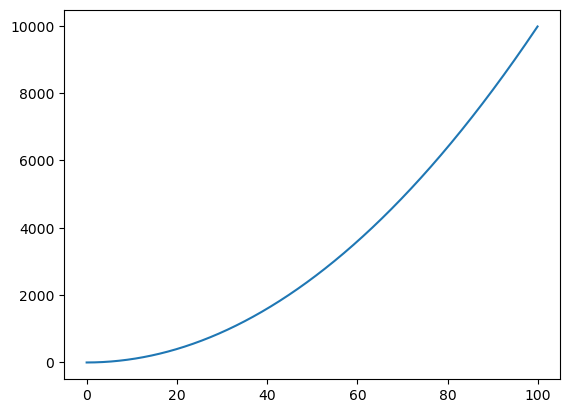
24,画图，y=x*x 其中 x = np.arange(0, 100, 0.1) （提示这里用到 matplotlib.pyplot 库）

# 24,画图，y=x*x 其中 x = np.arange(0, 100, 0.1) （提示这里用到  matplotlib.pyplot 库）
import matplotlib.pyplot as plt
x = np.arange(0, 100, 0.1)
y = x * x
plt.plot(x, y)
plt.show()

​

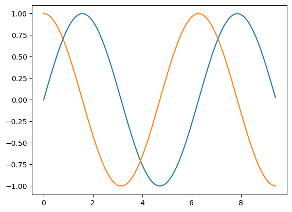
25.画图。画正弦函数和余弦函数， x = np.arange(0, 3 * np.pi, 0.1)(提示：这里用到 np.sin() np.cos() 函数和 matplotlib.pyplot 库)

# 25.画图。画正弦函数和余弦函数， x = np.arange(0, 3 * np.pi, 0.1)(提示：这里用到 np.sin() np.cos() 函数和 matplotlib.pyplot 库)
x = np.arange(0, 3 * np.pi, 0.1)
y1 = np.sin(x)
y2 = np.cos(x)
plt.plot(x, y1)
plt.plot(x, y2)
plt.show()

​

​

下面将详细介绍每个知识点的使用方法和操作技巧，并配合代码示例说明：

---

1. 导入库与基本设置

在使用 numpy 和 matplotlib 时，首先需要导入对应的库：

import numpy as np               # 导入 numpy 并简写为 np
import matplotlib.pyplot as plt  # 导入绘图库 matplotlib.pyplot，并简写为 plt

• numpy：主要用于数值计算和矩阵（数组）操作。
• matplotlib.pyplot：用于数据的可视化，常用于绘制各种图形。

---

2. 数组的创建与基本属性

数组的创建

• 一维数组：使用 np.array() 从列表创建。例如：

  a = np.array([4, 5, 6])
  

• 二维数组：直接嵌套列表创建。例如：

  b = np.array([[4, 5, 6], [1, 2, 3]])
  

数组的基本属性

• 类型：使用 type(a) 查看变量类型，结果通常为 <class 'numpy.ndarray'>。
• 形状（维度大小）：使用 a.shape 返回一个元组，表示各维度的大小。
• 数据类型：使用 a.dtype 得到数组中数据的类型（如 int32、float64）。

示例：

a = np.array([4, 5, 6])
print(type(a))   # <class 'numpy.ndarray'>
print(a.shape)   # (3,)
print(a.dtype)   # 例如 int32

---

3. 数组的索引与切片

基本索引

• 一维数组：通过下标访问单个元素，如 a[0] 得到第一个元素。

• 二维数组：通过 a[row, column] 访问。例如：

  b = np.array([[4, 5, 6], [1, 2, 3]])
  print(b[0, 0])  # 输出 4
  print(b[1, 1])  # 输出 2
  

切片操作

• 使用冒号 : 表示取范围。例如，从二维数组中取部分数据：

  a = np.array([[1, 2, 3, 4],
                [5, 6, 7, 8],
                [9, 10, 11, 12]])
  # 取第0、1行；第2、3列
  b = a[0:2, 2:4]
  print(b)  # 输出 [[3, 4], [7, 8]]
  

负数索引

• 使用 -1 可以表示倒数第一个元素。例如：

  print(b[0, -1])  # 输出第一行最后一个元素
  

花式索引（Fancy Indexing）

• 利用数组或列表作为索引，一次性选取多个任意位置的元素。例如：

  a = np.array([[1, 2], [3, 4], [5, 6]])
  # 分别选取 (0,0), (1,1), (2,0)
  print(a[[0, 1, 2], [0, 1, 0]])  # 输出 [1, 4, 5]
  

---

4. 特殊矩阵的生成

4.1 创建全零矩阵

• 使用 np.zeros(shape, dtype=...) 创建。例如：

  a = np.zeros((3, 3), dtype=int)
  

4.2 创建全一矩阵

• 使用 np.ones(shape) 创建。例如：

  b = np.ones((4, 5))
  

4.3 创建单位矩阵

• 使用 np.eye(n) 创建 n×n 的单位矩阵（对角线为1，其余为0）。

  c = np.eye(4)
  

4.4 生成随机数矩阵

• 使用 np.random.random(shape) 生成指定大小的随机浮点数矩阵，数值在0到1之间。

  d = np.random.random((3, 2))
  

---

5. 数组元素的修改

可以直接通过索引修改数组中某些元素的值。例如，下面代码将选定元素加上 10：

a = np.array([[1, 2, 3],
              [4, 5, 6],
              [7, 8, 9],
              [10, 11, 12]])
b = np.array([0, 2, 0, 1])
# np.arange(4) 得到 [0,1,2,3]，与 b 配合表示选取 (0,0), (1,2), (2,0), (3,1)
a[np.arange(4), b] += 10
print(a)

这种用法利用了花式索引，可以直接修改特定位置的元素。

---

6. 数组的数学运算

6.1 加法与减法

• 加法：可以使用 + 运算符或者 np.add()。
• 减法：可以使用 - 运算符或者 np.subtract()。

示例：

x = np.array([[1, 2], [3, 4]], dtype=np.float64)
y = np.array([[5, 6], [7, 8]], dtype=np.float64)

print(x + y)         # 使用 + 运算符
print(np.add(x, y))  # 使用 np.add()

print(x - y)         # 使用 - 运算符
print(np.subtract(x, y))  # 使用 np.subtract()

6.2 乘法与除法

• 元素乘法：使用 * 运算符或 np.multiply()。
• 矩阵乘法：使用 np.dot() 或 x.dot(y)，两者功能相同，但要注意形状匹配。
• 除法：使用 / 运算符或 np.divide()。

示例：

print(x * y)             # 元素乘法
print(np.multiply(x, y))  # 元素乘法
print(np.dot(x, y))       # 矩阵乘法

print(x / y)             # 元素除法
print(np.divide(x, y))    # 元素除法

6.3 开方和指数

• 开方：使用 np.sqrt() 计算数组中每个元素的平方根。
• 指数：使用 np.exp() 计算 e 的幂。

示例：

print(np.sqrt(x))
print(np.exp(x))

---

7. 数组的聚合操作

聚合操作用于对数组中所有或部分元素进行求和、求平均等操作。

7.1 求和

• 整体求和：np.sum(x) 将所有元素求和。
• 按轴求和：
  • np.sum(x, axis=0) 按列求和。
  • np.sum(x, axis=1) 按行求和。

示例：

print(np.sum(x))
print(np.sum(x, axis=0))
print(np.sum(x, axis=1))

7.2 求平均

• 整体平均：np.mean(x)。
• 按轴平均：
  • np.mean(x, axis=0) 按列求平均。
  • np.mean(x, axis=1) 按行求平均。

示例：

print(np.mean(x))
print(np.mean(x, axis=0))
print(np.mean(x, axis=1))

---

8. 数组的转置

数组转置可以通过 .T 属性实现，适用于二维数组。

示例：

print(x.T)

---

9. 数组中最大值的索引

利用 np.argmax() 可以找出数组中最大值的索引。对于多维数组，还可以指定轴。

示例：

print(np.argmax(x))          # 整个数组中最大元素的索引（按展平顺序）
print(np.argmax(x, axis=0))   # 每一列中最大值的索引
print(np.argmax(x, axis=1))   # 每一行中最大值的索引

---

10. 绘图操作

利用 matplotlib 绘图，可以将计算结果可视化。

10.1 绘制简单函数图像

例如绘制 ( y = x^2 )：

x = np.arange(0, 100, 0.1)  # 生成从 0 到 100 的数值，步长为 0.1
y = x * x                 # 计算 x 的平方
plt.plot(x, y)            # 绘制图形
plt.xlabel("x")
plt.ylabel("x^2")
plt.title("y = x^2")
plt.show()

10.2 绘制正弦和余弦函数

例如绘制正弦函数和余弦函数：

x = np.arange(0, 3 * np.pi, 0.1)
y1 = np.sin(x)
y2 = np.cos(x)
plt.plot(x, y1, label="sin(x)")
plt.plot(x, y2, label="cos(x)")
plt.xlabel("x")
plt.ylabel("y")
plt.title("正弦和余弦函数")
plt.legend()  # 显示图例
plt.show()

---

on
print(np.argmax(x)) # 整个数组中最大元素的索引（按展平顺序）
print(np.argmax(x, axis=0)) # 每一列中最大值的索引
print(np.argmax(x, axis=1)) # 每一行中最大值的索引

---

## 10. 绘图操作

利用 matplotlib 绘图，可以将计算结果可视化。

### 10.1 绘制简单函数图像

例如绘制 \( y = x^2 \)：

```python
x = np.arange(0, 100, 0.1)  # 生成从 0 到 100 的数值，步长为 0.1
y = x * x                 # 计算 x 的平方
plt.plot(x, y)            # 绘制图形
plt.xlabel("x")
plt.ylabel("x^2")
plt.title("y = x^2")
plt.show()

10.2 绘制正弦和余弦函数

例如绘制正弦函数和余弦函数：

x = np.arange(0, 3 * np.pi, 0.1)
y1 = np.sin(x)
y2 = np.cos(x)
plt.plot(x, y1, label="sin(x)")
plt.plot(x, y2, label="cos(x)")
plt.xlabel("x")
plt.ylabel("y")
plt.title("正弦和余弦函数")
plt.legend()  # 显示图例
plt.show()

---