当前位置：首页 > news >正文

《强量化 Transformers：开启计算机视觉新篇》

news 2025/11/15 7:43:20

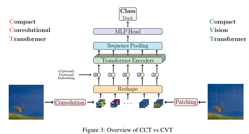
一、Compact Convolutional Transformers

ViT在小型数据集上性能不够好的问题，这个问题非常实际，现实情况下如果确实没有大量数据集，同时也没有合适的预训练模型需要从头训练的时候，ViT架构性能是不如CNN架构的。这篇文章实际上并没有引入大量的卷积操作，通过修改patch size，以及使用SeqPool的方法就可以取得不错的成绩。

CCT 的核心设计理念是将卷积神经网络强大的局部特征提取能力与 Transformer 卓越的全局建模能力深度融合，兼收并蓄两者之长。通过精心设计的卷积模块，CCT 能够高效地提取图像中的局部细节信息，精准捕捉图像中物体的边缘、纹理等特征；而 Transformer 模块则负责在更大的范围内建模，捕捉不同局部区域之间的长距离依赖关系，从而对图像的整体结构和语义有更全面、深入的理解。

核心贡献如下：

通过引入ViT-Lite能够有效从头开始在小型数据集上实现更高精度，打破Transformer需要大量数据的神话。
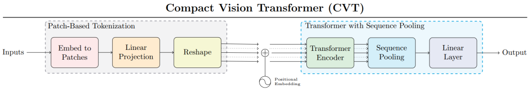
引入新型序列池化策略（sequence pooling)的CVT（Compact Vision Transformer），从而让Transformer无需class token
引入CCT（Compact Convolutional Transformer）来提升模型性能，同时可以让图片输入尺寸更加灵活。

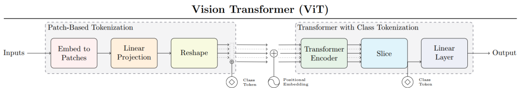
(1) ViT-Lite

(2) CVT

(3)CCT

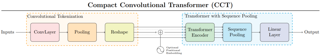
与传统 ViT 中简单粗暴地将图像分割成均匀、非重叠的补丁不同，CCTTokenizer 引入了一个全卷积迷你网络.每一层卷积都像是在对图像进行一次深度的 "扫描"，提取出不同层次的特征；零填充层巧妙地保持了图像的空间尺寸，确保信息的完整性；而最大池化层则在降低数据维度的同时，突出了图像中的关键特征。

CCT 模型构建与训练

（一）数据预处理与增强

在 CCT 模型的训练征程中，数据预处理与增强是至关重要的起始步骤，如同精心准备食材是烹饪出美味佳肴的基础。本次实验选用的 CIFAR - 10 数据集，宛如一座丰富的图像宝库，其中包含了 10 个不同类别的 60000 张彩色图像，每类图像各有 6000 张，这些图像如同繁星般璀璨，涵盖了飞机、汽车、鸟类、猫、鹿、狗、青蛙、马、船和卡车等众多物体，为模型的训练提供了丰富多样的样本。

(二)模型的搭建（keras)

import tensorflow as tf
from keras import layers
import kerasimport matplotlib.pyplot as plt
import numpy as np'''导入需要的模块''''''超参数设置'''
positional_emb = True
conv_layers = 2
projection_dim = 128num_heads = 2
transformer_units = [projection_dim,projection_dim,
]
transformer_layers = 2
stochastic_depth_rate = 0.1learning_rate = 0.001
weight_decay = 0.0001
batch_size = 128
num_epochs = 30
image_size = 32'''数据集下载---cifar10'''
num_classes = 10
input_shape = (32, 32, 3)(x_train, y_train), (x_test, y_test) = keras.datasets.cifar10.load_data()y_train = keras.utils.to_categorical(y_train, num_classes)
y_test = keras.utils.to_categorical(y_test, num_classes)print(f"x_train shape: {x_train.shape} - y_train shape: {y_train.shape}")
print(f"x_test shape: {x_test.shape} - y_test shape: {y_test.shape}")'''CCT token'''class CCTTokenizer(layers.Layer):def __init__(self,kernel_size=3,stride=1,padding=1,pooling_kernel_size=3,pooling_stride=2,num_conv_layers=conv_layers,num_output_channels=[64, 128],positional_emb=positional_emb,**kwargs,):super().__init__(**kwargs)# This is our tokenizer.self.conv_model = keras.Sequential()for i in range(num_conv_layers):self.conv_model.add(layers.Conv2D(num_output_channels[i],kernel_size,stride,padding="valid",use_bias=False,activation="relu",kernel_initializer="he_normal",))self.conv_model.add(layers.ZeroPadding2D(padding))self.conv_model.add(layers.MaxPooling2D(pooling_kernel_size, pooling_stride, "same"))self.positional_emb = positional_embdef call(self, images):outputs = self.conv_model(images)# After passing the images through our mini-network the spatial dimensions# are flattened to form sequences.batch_size = tf.shape(outputs)[0]h = tf.shape(outputs)[1]w = tf.shape(outputs)[2]c = tf.shape(outputs)[3]reshaped = tf.reshape(outputs,(batch_size, h * w, c))return reshaped'''位置编码'''class PositionEmbedding(keras.layers.Layer):def __init__(self,sequence_length,initializer="glorot_uniform",**kwargs,):super().__init__(**kwargs)if sequence_length is None:raise ValueError("`sequence_length` must be an Integer, received `None`.")self.sequence_length = int(sequence_length)self.initializer = keras.initializers.get(initializer)def get_config(self):config = super().get_config()config.update({"sequence_length": self.sequence_length,"initializer": keras.initializers.serialize(self.initializer),})return configdef build(self, input_shape):feature_size = input_shape[-1]self.position_embeddings = self.add_weight(name="embeddings",shape=[self.sequence_length, feature_size],initializer=self.initializer,trainable=True,)super().build(input_shape)def call(self, inputs, start_index=0):shape = tf.shape(inputs)feature_length = shape[-1]sequence_length = shape[-2]# trim to match the length of the input sequence, which might be less# than the sequence_length of the layer.position_embeddings = tf.convert_to_tensor(self.position_embeddings)position_embeddings = tf.slice(position_embeddings,[start_index, 0],[sequence_length, feature_length],)return tf.broadcast_to(position_embeddings, shape)def compute_output_shape(self, input_shape):return input_shapeclass SequencePooling(layers.Layer):def __init__(self):super().__init__()self.attention = layers.Dense(1)def call(self, x):attention_weights = tf.nn.softmax(self.attention(x), axis=1)attention_weights = tf.transpose(attention_weights, perm=(0, 2, 1))weighted_representation = tf.matmul(attention_weights, x)return tf.squeeze(weighted_representation, -2)class StochasticDepth(layers.Layer):def __init__(self, drop_prop, **kwargs):super().__init__(**kwargs)self.drop_prob = drop_propdef call(self, x, training=None):if training:keep_prob = 1 - self.drop_probshape = (tf.shape(x)[0],) + (1,) * (len(x.shape) - 1)random_tensor = keep_prob + tf.random.uniform(shape, 0, 1)random_tensor = tf.floor(random_tensor)return (x / keep_prob) * random_tensorreturn xdef mlp(x, hidden_units, dropout_rate):for units in hidden_units:x = layers.Dense(units, activation=tf.nn.gelu)(x)x = layers.Dropout(dropout_rate)(x)return xdata_augmentation = keras.Sequential([layers.Rescaling(scale=1.0 / 255),layers.RandomCrop(image_size, image_size),layers.RandomFlip("horizontal"),],name="data_augmentation",
)def create_cct_model(image_size=image_size,input_shape=input_shape,num_heads=num_heads,projection_dim=projection_dim,transformer_units=transformer_units,
):inputs = layers.Input(input_shape)# Augment data.augmented = data_augmentation(inputs)# Encode patches.cct_tokenizer = CCTTokenizer()encoded_patches = cct_tokenizer(augmented)# Apply positional embedding.if positional_emb:sequence_length = encoded_patches.shape[1]encoded_patches += PositionEmbedding(sequence_length=sequence_length)(encoded_patches)# Calculate Stochastic Depth probabilities.dpr = [x for x in np.linspace(0, stochastic_depth_rate, transformer_layers)]# Create multiple layers of the Transformer block.for i in range(transformer_layers):# Layer normalization 1.x1 = layers.LayerNormalization(epsilon=1e-5)(encoded_patches)# Create a multi-head attention layer.attention_output = layers.MultiHeadAttention(num_heads=num_heads, key_dim=projection_dim, dropout=0.1)(x1, x1)# Skip connection 1.attention_output = StochasticDepth(dpr[i])(attention_output)x2 = layers.Add()([attention_output, encoded_patches])# Layer normalization 2.x3 = layers.LayerNormalization(epsilon=1e-5)(x2)# MLP.x3 = mlp(x3, hidden_units=transformer_units, dropout_rate=0.1)# Skip connection 2.x3 = StochasticDepth(dpr[i])(x3)encoded_patches = layers.Add()([x3, x2])# Apply sequence pooling.representation = layers.LayerNormalization(epsilon=1e-5)(encoded_patches)weighted_representation = SequencePooling()(representation)# Classify outputs.logits = layers.Dense(num_classes)(weighted_representation)# Create the Keras model.model = keras.Model(inputs=inputs, outputs=logits)return modeldef run_experiment(model):optimizer = keras.optimizers.AdamW(learning_rate=0.001, weight_decay=0.0001)model.compile(optimizer=optimizer,loss=keras.losses.CategoricalCrossentropy(from_logits=True, label_smoothing=0.1),metrics=[keras.metrics.CategoricalAccuracy(name="accuracy"),keras.metrics.TopKCategoricalAccuracy(5, name="top-5-accuracy"),],)checkpoint_filepath = "/tmp/checkpoint.weights.h5"checkpoint_callback = keras.callbacks.ModelCheckpoint(checkpoint_filepath,monitor="val_accuracy",save_best_only=True,save_weights_only=True,)history = model.fit(x=x_train,y=y_train,batch_size=batch_size,epochs=num_epochs,validation_split=0.1,callbacks=[checkpoint_callback],)model.load_weights(checkpoint_filepath)_, accuracy, top_5_accuracy = model.evaluate(x_test, y_test)print(f"Test accuracy: {round(accuracy * 100, 2)}%")print(f"Test top 5 accuracy: {round(top_5_accuracy * 100, 2)}%")return historycct_model = create_cct_model()
history = run_experiment(cct_model)

模型性能
根据中的实现和注释，CCT 模型在 CIFAR-10 数据集上展现出了高效的性能：

参数量：约 40 万参数，仅为标准 ViT 的 9%
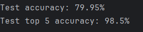
准确率：在 30 个 epoch 训练后达到约 79% 的 top-1 准确率
训练速度：由于参数量少，训练速度快，适合在有限计算资源上运行

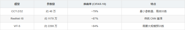
需要注意的是，CCT 模型的设计重点是参数效率，而不是绝对性能。在资源受限的环境中，CCT 提供了很好的性能和资源消耗平衡。

参考

https://arxiv.org/abs/2104.05704

https://github.com/SHI-Labs/Compact-Transformers

https://zhuanlan.zhihu.com/p/364589899

二 MobileViT: Light-weight, General-purpose, and Mobile-friendly Vision Transformer

论文地址：https://arxiv.org/pdf/2110.02178

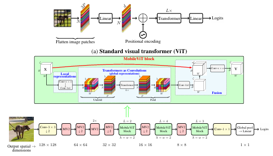
它可以有效地将局部和全局信息进行编码。与ViT及其变体不同，MobileViT从不同的角度学习全局表示。标准卷积涉及三个操作：展开（unfloading） 、局部处理（local processing） 和展开（folding） 。MobileViT块使用Transformer将卷积中的局部建模替换为全局建模。这使得MobileViT块具有CNN和ViT的性质，有助于它用更少的参数和简单的训练方式学习更好的表示。

查看全文

http://www.dtcms.com/a/609851.html