TensorFlow 2.x常用函数总结(持续更新)
本文主要记录自己在用 Tensorflow 2.x 复现经典模型过程中遇到的一些函数及用法,方便查阅
目录
tf 2.x 常用函数
tf.zeros_like()
tf.ones() / tf.ones_like()
tf.cast()
tf.equal() / tf.not_equal()
tf.logical_or() / tf.logical_and() / tf.logical_not()
tf.greater() / tf.less()
tf.sign()
tf.clip_by_value()
tf.identity()
tf.fill()
tf.size()
tf.squeeze() / tf.unsqueeze()
tf.where()
tf.cond()
tf.concat()
tf.stack()
tf.reduce_mean() / tf.reduce_sum() / tf.reduce_max()
tf.reduce_all() / tf.reduce_any()
tf.tile()
tf.boolean_mask()
tf.gather() / tf.gather_nd()
tf.scatter_nd()
tf.slice()
tf.multiply() / *
tf.matmul() / @
tf.transpose()
tf.add_n()
tf.divide()
tf.maximum() / tf.reduce_max()
tf.math.subtract()
tf.pow() / tf.exp() / tf.abs()
tf.math.rint()
tf.math.log1p()
tf.nn.l2_normalize()
tf.nn.relu()
tf.random.normal()
tf.expand_dims()
tf.reshape()
tf.range()
tf.sequence_mask()
tf.nn.embedding_lookup()
其他常用
class、__init__、call
assign_sub / assign
tf.float32.min
logging.info()
tf 2.x 常用函数
tf.zeros_like()
用于生成一个和输入张量(tensor)具有相同形状和数据类型、但所有元素都是零的新张量
import tensorflow as tf# 创建一个张量
tensor = tf.constant([[1, 2, 3], [4, 5, 6]])# 使用 tf.zeros_like() 创建一个和上面张量相同形状和数据类型的全零张量
zero_tensor = tf.zeros_like(tensor)
print(zero_tensor)
输出结果为:
tf.Tensor(
[[0 0 0][0 0 0]], shape=(2, 3), dtype=int32)
同理,若创建全1张量,函数为tf.ones_like()
tf.ones() / tf.ones_like()
它们的主要作用都是生成元素全为1的张量,但存在一些区别:
tf.ones()需要一个形状为参数,然后返回一个与给定形状相匹配的、全是1的新张量tf.ones_like()需要一个已存在的张量作为参数,然后返回一个与给定张量形状相同的、全是1的新张量,无需手动指定形状
import tensorflow as tfa = tf.ones((2, 3))    # 输出一个形状为(2,3)、元素全为1的张量
print(a)# 输出一个与tensor形状相同、元素全为1的新张量
tensor = tf.constant([[1, 2, 3], [4, 5, 6]])
b = tf.ones_like(tensor)
print(b)总的来说,tf.ones() 需要手动指定形状,而 tf.ones_like() 则是根据已存在的张量的形状来创建新的元素全为1的张量
tf.cast()
用来改变Tensor的数据类型。如果在转换过程中,原Tensor的数值无法适应新的数据类型,则会产生一定形式的截断
- 输入:待转换的Tensor以及目标数据类型
- 输出:一个新的数据类型转换后的Tensor
import tensorflow as tf# 创建一个float类型的Tensor
x = tf.constant([1.8, 2.2], dtype=tf.float32)# 使用cast函数将其转换为int32类型的Tensor
x_cast = tf.cast(x, tf.int32)
print(x_cast)
输出结果为:
tf.Tensor([1 2], shape=(2,), dtype=int32)可以看到,小数部分被截断,只保留整数部分,这就是tf.cast函数的数据类型转换功能
tf.equal() / tf.not_equal()
tf.equal()函数是用来比较两个具有相同维度和形状的tensor中的对应元素是否相等。会逐元素地进行比较,如果对应位置的元素相等返回True,否则返回False
import tensorflow as tf# 创建两个tensor
tensor1 = tf.constant([1, 2, 3, 4])
tensor2 = tf.constant([1, 2, 3, 5])# 返回一个布尔型张量,其中每个元素代表了相应位置的元素是否相等
equal_comparison = tf.equal(tensor1, tensor2)
print(equal_comparison)
输出结果为:
tf.Tensor([ True True True False], shape=(4,), dtype=bool)tf.not_equal()函数则相反,用于判断两个张量中的元素是否不相等。若对应位置元素不相等返回True,否则返回False
import tensorflow as tf# 创建两个tensor
tensor1 = tf.constant([1, 2, 3, 4])
tensor2 = tf.constant([2, 2, 3, 3])equal_comparison = tf.not_equal(tensor1, tensor2)
print(equal_comparison)
输出结果为:
tf.Tensor([ True False False True], shape=(4,), dtype=bool)tf.logical_or() / tf.logical_and() / tf.logical_not()
tf.logical_or()用于执行元素级的逻辑或运算(只要有一个True就返回True)
- 输入:两个布尔类型的张量
- 输出:一个布尔类型张量,每一个元素都是对应位置上的两个元素的逻辑或结果
import tensorflow as tf# 创建两个布尔型张量
tensor1 = tf.constant([True, False, True, False])
tensor2 = tf.constant([False, False, True, True])result = tf.logical_or(tensor1, tensor2)
print(result)
输出结果为:
tf.Tensor([ True False True True], shape=(4,), dtype=bool)
tf.logical_and() 和 tf.logical_not() 同理,分别是逻辑与(全为True才返回True)、逻辑非(取反)运算
- 逻辑与
tf.logical_and()
import tensorflow as tf# 创建两个布尔型张量
tensor1 = tf.constant([True, False, True, False])
tensor2 = tf.constant([True, True, False, False])result = tf.logical_and(tensor1, tensor2)
print(result)
输出结果为:
tf.Tensor([ True False False False], shape=(4,), dtype=bool)
- 逻辑非
tf.logical_not():输入是一个或多个布尔值的张量,输出是一个同维度的布尔张量
import tensorflow as tf# 创建一个布尔型的张量
bool_tensor = tf.constant([True, False, True, False])tensor = tf.logical_not(bool_tensor)
print(tensor)
输出结果为:
tf.Tensor([False True False True], shape=(4,), dtype=bool)tf.greater() / tf.less()
tf.greater()用于执行元素级别的大于比较
- 输入:两个需要比较大小的tensor
- 输出:一个与输入相同形状的新的布尔型tensor。其中每一个元素表示在对应位置上,第一个tensor中的元素是否大于第二个tensor中的元素,大于则为True,否则为False
import tensorflow as tfa = tf.constant([1, 2, 3])
b = tf.constant([2, 2, 2])result = tf.greater(a, b)
print(result)
输出结果为:
tf.Tensor([False False True], shape=(3,), dtype=bool)
tf.less()同理,进行元素级别的小于比较
import tensorflow as tfa = tf.constant([1, 2, 3])
b = tf.constant([2, 2, 2])result = tf.less(a, b)
print(result)
输出结果为:
tf.Tensor([True False False], shape=(3,), dtype=bool)
tf.sign()
tf.sign()将输入张量中的正数转换为1,负数转换为-1,而 0 则保持不变。返回的张量与输入的张量形状相同
import tensorflow as tfx = tf.constant([1.8, -2.2, 0, -3.3, 2.5], dtype=tf.float32)x_sign = tf.sign(x)
print(x_sign)
输出结果为:
tf.Tensor([ 1. -1. 0. -1. 1.], shape=(5,), dtype=float32)tf.clip_by_value()
tf.clip_by_value()用于将张量中的数值限制在某个范围内。这个函数的标准使用方法如下:
tf.clip_by_value(t, clip_value_min, clip_value_max)在这里,t是待截取的张量,clip_value_min 和 clip_value_max 则分别是待截取范围的最小值和最大值。函数返回一个新的、按指定的最小值和最大值截取的张量
import tensorflow as tft = tf.constant([0.9, 2.5, 3.3, 4.5])clip_t = tf.clip_by_value(t, 1.0, 3.0)
print(clip_t)
输出结果为:
tf.Tensor([1. 2.5 3. 3. ], shape=(4,), dtype=float32)tf.clip_by_value()在训练深度学习模型时非常实用。例如在训练神经网络时,可以用这个函数来防止梯度消失或爆炸,使学习率保持在一个合理的范围内
tf.identity()
tf.identity()用于创建一个与输入tensor相同的新tensor(独立于输入tensor)
import tensorflow as tfx = tf.constant([2, 3, 4])
y = tf.identity(x)    # y被定义为x的副本,但独立于x,即对y的操作不会影响xprint("x: ", x)
print("y: ", y)
输出结果为:
x:  tf.Tensor([2 3 4], shape=(3,), dtype=int32)
y:  tf.Tensor([2 3 4], shape=(3,), dtype=int32)
一个使用 tf.identity()的常见场景是为 tensor 添加一个名称(可以帮助我们在复杂的神经网络中更好地追踪和调试tensor),如:
x = tf.constant([2, 3, 4])y = tf.identity(x, name="my_tensor")
print("y: ", y)    # 输出结果同上
tf.fill()
tf.fill()作用是创建一个指定维度和数值的张量
tf.fill(dims, value)其中 dims 是一个列表,代表了想要创建的张量的形状;value 是想要填充的值
import tensorflow as tf# 创建一个形状为[2,3],所有元素值为9的张量
a = tf.fill([2, 3], 9)
print(a)
输出结果为:
tf.Tensor(
[[9 9 9][9 9 9]], shape=(2, 3), dtype=int32)
tf.size()
tf.size()函数返回的是一个Scalar Tensor,即一个单一数值,表示输入Tensor 包含的元素个数,为所有维度大小的乘积
import tensorflow as tfa = tf.constant([[1, 2, 3], [4, 5, 6]])   # 形状是(2,3)
print(tf.size(a))   # 返回 6 = 2 * 3
输出结果为:
tf.Tensor(6, shape=(), dtype=int32)tf.squeeze() / tf.unsqueeze()
tf.squeeze()作用是从张量中移除所有长度为1的维度。例如,如果有一个形状为 [1, 3, 1, 4, 1] 的张量,使用 tf.squeeze()函数后,会得到一个形状为 [3, 4] 的张量
需要注意的是,tf.squeeze()函数默认会移除所有长度为1的维度。如果只想移除特定的长度为1的维度,可以通过 axis 参数指定。例如,tf.squeeze(tensor, axis=[2, 4]) 只会移除第2和第4维(从0开始计数)
import tensorflow as tf# 创建一个形状为 [1, 3, 1, 4, 1] 的张量
tensor = tf.ones([1, 3, 1, 4, 1])# 使用 tf.squeeze 并指定axis 移除特定的长度为1的维度
squeezed_tensor = tf.squeeze(tensor, axis=[2, 4])
print(squeezed_tensor.shape)
输出结果为:
(1, 3, 4)注:逆操作为 tf.unsqueeze()
tf.where()
tf.where()函数主要用于根据条件选择元素或获取张量中非零元素的索引
(1)根据条件选择元素:tf.where(condition, x, y)
- 根据
condition从x和y中选择元素,当condition为 True 时,选择x中对应位置的元素;当condition为 False 时,选择y中对应位置的元素 - 返回 tensor 与
condition的 shape 是相同的 - 支持广播,当
x和y的形状与condition不匹配时会自动广播
import tensorflow as tfcondition = tf.constant([[True, False], [False, True]])
x = tf.constant([[1, 2], [3, 4]])
y = tf.constant([[10, 20], [30, 40]])result = tf.where(condition, x, y)
print(result.numpy())
输出结果为:
[[ 1 20][30 4]](2)获取非零元素的索引:tf.where(condition)
-
返回
condition中为 True 的元素的索引,返回张量的形状为[num_true, rank]
import tensorflow as tf# 一维示例
tensor = tf.constant([0, 5, 0, 8, 0, 3])
indices = tf.where(tensor)
print(indices.numpy())# 二维示例
matrix = tf.constant([[0, 1, 0],[1, 0, 1],[0, 0, 1]])
indices_2d = tf.where(matrix)
print(indices_2d.numpy())
输出结果为:
[[1][3][5]][[0 1][1 0][1 2][2 2]]对比 tf.where() 和 tf.boolean_mask():
# 相同的数据过滤,boolean_mask vs where 两种方法对比
tensor = tf.constant([1, 2, 3, 4, 5])
mask = tf.constant([True, False, True, False, True])# 使用 boolean_mask
result_mask = tf.boolean_mask(tensor, mask)
print("boolean_mask 结果:", result_mask.numpy())  # [1 3 5]# 使用 where 实现相同功能
indices = tf.where(mask)
print(indices)
# tf.Tensor([[0]
#            [2]
#            [4]], shape=(3, 1), dtype=int64)print(indices[:, 0])   # tf.Tensor([0 2 4], shape=(3,), dtype=int64)result_where = tf.gather(tensor, indices[:, 0])
print("where+gather 结果:", result_where.numpy())  # [1 3 5]
tf.cond()
用于条件执行的控制流函数,根据条件选择执行两个不同计算分支中的一个
tf.cond(pred, true_fn, false_fn, name=None)pred:标量布尔张量,决定执行哪个分支,且两个分支必须返回相同的数据类型和形状true_fn:可调用函数,当pred为 True 时执行false_fn:可调用函数,当pred为 False 时执行
# 如果 x 等于 y,则操作返回 x + z 的值,否则返回 y 的平方值
result = tf.cond(tf.equal(x, y), lambda: tf.add(x, z), lambda: tf.square(y))
应用:梯度裁剪(Gradient Clipping。作用是防止梯度爆炸,通过限制梯度大小来稳定训练过程)
import tensorflow as tf# 根据梯度大小决定是否进行梯度裁剪
gradients = tf.constant([1.5, -2.3, 0.8, 4.1])
max_grad_norm = 2.0   # 最大梯度范数阈值# 计算梯度的L2范数(欧几里得范数)
grad_norm = tf.sqrt(tf.reduce_sum(tf.square(gradients)))
# 等价于:||gradients||₂ = √(Σ gradientᵢ²)def clip_fn():# 需要裁剪的情况scale = max_grad_norm / grad_norm   # 缩放比例return gradients * scale   # 按比例缩放梯度def no_clip_fn():# 不需要裁剪的情况return gradientsclipped_gradients = tf.cond(grad_norm > max_grad_norm, clip_fn, no_clip_fn)
与 tf.where() 相比,tf.cond() 真正控制计算图的执行路径,而 tf.where() 会计算所有分支然后选择结果。这使得 tf.cond() 在需要避免不必要计算时更加高效
tf.concat()
tf.concat()函数用于将两个或更多的张量沿特定的轴连接(拼接)在一起,前提条件是拼接的张量具有相同的数据类型,且在非连接轴上的维度必须相同
tf.concat(values, axis, name=None)values:要连接的张量列表或元组axis:axis=0(行)为纵向拼接,axis=1(列)为横向拼接。默认axis=0name:操作的名称(可选)
import tensorflow as tf### 一维示例 ###
t1 = tf.constant([1, 2, 3])
t2 = tf.constant([4, 5, 6])# 沿着第0维连接(默认)
result0 = tf.concat([t1, t2], axis=0)
print(result0.numpy())  # 输出: [1 2 3 4 5 6]### 二维示例 ###
a = tf.constant([[1, 2, 3],[4, 5, 6]])
b = tf.constant([[7, 8, 9],[10, 11, 12]])# 沿着第0维连接(垂直堆叠)
result_0 = tf.concat([a, b], axis=0)
print(result_0.numpy())
# 输出:
# [[ 1  2  3]
#  [ 4  5  6]
#  [ 7  8  9]
#  [10 11 12]]# 沿着第1维连接(水平堆叠)
result_1 = tf.concat([a, b], axis=1)
print(result_1.numpy())
# 输出:
# [[ 1  2  3  7  8  9]
# [ 4 5 6 10 11 12]]三维及以上张量拼接的维度变化:如两个 shape 为 (2, 2, 2) 的三维张量做连接。若axis=0,则输出 shape 为 (4, 2, 2);若axis=1,则输出 shape 为 (2, 4, 2);若axis=2,则输出 shape 为 (2, 2, 4)
与tf.stack()函数的区别:
import tensorflow as tfa = tf.constant([1, 2, 3])
b = tf.constant([4, 5, 6])concat_result = tf.concat([a, b], axis=0)  # 形状: (6,)
stack_result = tf.stack([a, b], axis=0)    # 形状: (2, 3)print("concat 结果: \n", concat_result)
print("stack 结果: \n", stack_result)
输出结果为:
concat 结果: tf.Tensor([1 2 3 4 5 6], shape=(6,), dtype=int32)stack 结果: tf.Tensor(
[[1 2 3][4 5 6]], shape=(2, 3), dtype=int32)
tf.stack()
tf.stack()是一个用于将多个张量沿新维度堆叠的操作。它的功能类似于numpy中的np.stack(),能够将一组相同形状的张量合并为一个更高维的张量
tf.stack(values, axis=0, name='stack')- 参数:
values:一个张量列表(所有张量必须有相同的形状和数据类型)axis:指定堆叠的维度(默认为0,即第一个维度)name:操作的名称(可选)
- 返回:堆叠后的新张量,比输入张量多一个维度
import tensorflow as tf# 定义两个形状相同的张量
x = tf.constant([1, 2, 3])  # shape: (3,)
y = tf.constant([4, 5, 6])  # shape: (3,)# 沿 axis=0 堆叠(默认)
stacked = tf.stack([x, y])   # shape: (2, 3)
print(stacked.numpy())
# 输出:
# [[1 2 3]
#  [4 5 6]]# 沿 axis=1 堆叠
stacked = tf.stack([x, y], axis=1)  # shape: (3, 2)
print(stacked.numpy())
# 输出:
# [[1 4]
#  [2 5]
#  [3 6]]
与 tf.concat() 的区别:
| 操作 | 行为 | 示例输入shape [2,3], [2,3] | 输出形状 |
|---|---|---|---|
tf.stack | 新增维度堆叠 | 将两个矩阵堆叠为一个三维张量 | [2, 2, 3](axis=0) |
tf.concat | 沿现有维度拼接 | 将两个矩阵上下拼接为一个大矩阵 | [4, 3](axis=0) |
tf.reduce_mean() / tf.reduce_sum() / tf.reduce_max()
tf.reduce_mean()是一个归约操作(reduction operation),用于计算张量沿指定维度的平均值
tf.reduce_mean(input_tensor,axis=None,keepdims=False,name=None
)| 参数 | 类型 | 说明 |
|---|---|---|
input_tensor | Tensor | 输入张量(必须是数值类型:float16, float32, int32 等) |
axis | int/list/None | 要归约的维度(默认为 None,计算所有元素的均值) |
keepdims | bool | 是否保留原始维度(默认为 False,降维) |
name | str | 操作的名称(可选) |
axis=0表示沿每一列(垂直轴)的方向求均值,axis=1表示沿每一行(水平轴)的方向求均值
返回值:沿指定维度求均值后的张量(维度根据 keepdims 决定)
import tensorflow as tf### 计算全局均值 ###
x = tf.constant([[1., 2.], [3., 4.]])
mean_all = tf.reduce_mean(x)  # (1+2+3+4)/4 = 2.5
print(mean_all)  # tf.Tensor(2.5, shape=(), dtype=float32)### 沿特定轴求均值 ###
# 沿 axis=0(列方向)
mean_col = tf.reduce_mean(x, axis=0)  # [(1+3)/2, (2+4)/2] = [2., 3.]
print(mean_col)  # tf.Tensor([2. 3.], shape=(2,), dtype=float32)# 沿 axis=1(行方向)
mean_row = tf.reduce_mean(x, axis=1)  # [(1+2)/2, (3+4)/2] = [1.5 3.5]
print(mean_row)  # tf.Tensor([1.5 3.5], shape=(2,), dtype=float32)# keepdims=True
mean_row = tf.reduce_mean(x, axis=1, keepdims=True)  # [[(1+2)/2], [(3+4)/2]]
print(mean_row) # tf.Tensor([[1.5], [3.5]], shape=(2, 1), dtype=float32)三维及以上张量归约:如输入 shape 为 (1, 2, 3),归约的轴为 axis=-1,则输出 shape 为 (1, 2)
tf.reduce_sum() / tf.reduce_max():
tf.reduce_sum()类似,用于计算张量在指定轴上的元素之和tf.reduce_max()沿着指定维度计算张量的最大值(输出维度会减少除非 keepdims=True)
# 找到概率最大的类别
def predict_class(probabilities):"""预测类别 - 找到最大概率的索引"""max_prob = tf.reduce_max(probabilities, axis=1)  # 每行的最大值predicted_class = tf.argmax(probabilities, axis=1)  # 最大值的索引return max_prob, predicted_class
tf.reduce_all() / tf.reduce_any()
执行逻辑与(AND)归约,即沿着指定的维度计算所有元素的逻辑与
tf.reduce_all(input_tensor, axis=None, keepdims=False, name=None)input_tensor:输入布尔张量axis:要归约的维度,如果为 None 则归约所有维度(axis=1表示沿行归约,axis=0表示沿列归约)keepdims:如果为 True,保留长度为1的维度
import tensorflow as tf# 一维张量归约
tensor_1d = tf.constant([True, True, False, True])
result = tf.reduce_all(tensor_1d)
print(result.numpy())  # False# 二维张量归约
matrix = tf.constant([[True, True, True],[True, False, True],[True, True, True]])# 归约所有元素
all_elements = tf.reduce_all(matrix)
print("所有元素都为True:", all_elements.numpy())  # False
# 等价于多轴归约 tf.reduce_all(matrix, axis=[0, 1])# 沿行归约(检查每行是否全为True)
all_per_row = tf.reduce_all(matrix, axis=1)
print("每行是否全为True:", all_per_row.numpy())  # [ True False  True]# 沿列归约(检查每列是否全为True)
all_per_col = tf.reduce_all(matrix, axis=0)
print("每列是否全为True:", all_per_col.numpy())  # [ True False  True]# keepdims=True
result_keepdims = tf.reduce_all(matrix, axis=1, keepdims=True)
print(result_keepdims)
# tf.Tensor(
# [[ True]
#  [False]
#  [ True]], shape=(3, 1), dtype=bool)
特殊情况:
- 空张量的
reduce_all返回True -
数值张量中0为False,非0为True
对比 tf.reduce_any():
reduce_all (逻辑与):所有元素都为True
reduce_any (逻辑或):至少一个元素为True
tf.tile()
tf.tile()函数用于张量平铺(复制),通过沿指定维度复制张量来扩展张量的大小
tf.tile(input, multiples, name=None)input:要平铺的输入张量multiples:一个1维整数张量,指定每个维度复制的次数name:操作的名称(可选)
import tensorflow as tf### 一维示例 ###
tensor_1d = tf.constant([1, 2, 3])    # shape=(3,)# 沿第0维复制2次
tiled_1d = tf.tile(tensor_1d, multiples=[2])
print(tiled_1d.numpy())   # [1 2 3 1 2 3]  shape=(6,)# 同时沿行和列复制
tiled_1d = tf.tile(tensor_1d, multiples=[2, 1])
print(tiled_1d.numpy())   # shape=(2, 3)
# [[1, 2, 3],
#  [1, 2, 3]]### 二维示例 ###
matrix = tf.constant([[1, 2],[3, 4]])# 沿行方向复制2次(axis=0)
tiled_rows = tf.tile(matrix, multiples=[2, 1])
print(tiled_rows.numpy())
# [[1 2]
#  [3 4]
#  [1 2]
#  [3 4]]# 沿列方向复制3次(axis=1)
tiled_cols = tf.tile(matrix, multiples=[1, 3])
print(tiled_cols.numpy())
# [[1 2 1 2 1 2]
#  [3 4 3 4 3 4]]# 同时沿行和列复制
tiled_both = tf.tile(matrix, multiples=[2, 3])
print(tiled_both.numpy())
# [[1 2 1 2 1 2]
#  [3 4 3 4 3 4]
#  [1 2 1 2 1 2]
# [3 4 3 4 3 4]]三维及以上张量平铺:如 shape 为 (1, 2, 2) 的 input,当 multiples=[2, 1, 1] 时,输出 shape 为 (2, 2, 2);当 multiples=[2, 2, 3] 时,输出 shape 为 (2, 4, 6)
-
multiples=[a, b, c] 表示第0维复制a次、第1维复制b次、第2维复制c次
常用于批次数据扩展,如:
batch_data = tf.tile(single_sample, multiples=[batch_size, 1])
tf.boolean_mask()
tf.boolean_mask()函数由给定布尔掩码、根据特定轴、从输入张量中提取元素、组成新张量
tf.boolean_mask(tensor, mask, axis=None, name=None)-
mask:布尔类型的张量,形状必须与tensor的前若干个维度兼容。True代表保留tensor中相应位置的元素,False代表舍弃 -
axis:可选的轴,指定应用掩码的维度。默认沿第一个维度(行)应用掩码
import tensorflow as tf### 一维示例 ###
tensor_1d = tf.constant([1, 2, 3, 4, 5])
mask_1d = tf.constant([True, False, True, False, True])result = tf.boolean_mask(tensor_1d, mask_1d)
print(result.numpy())    # [1 3 5]### 二维示例 ###
matrix = tf.constant([[1, 2, 3],[4, 5, 6],[7, 8, 9]])
mask_2d = tf.constant([True, False, True])# 默认沿第一个维度(行)应用掩码
result = tf.boolean_mask(matrix, mask_2d)
print(result.numpy())
# [[1 2 3]
#  [7 8 9]]# 沿特定轴应用掩码
result = tf.boolean_mask(matrix, mask_2d, axis=1)
print(result.numpy())
# [[1 3]
#  [4 6]
#  [7 9]]
三维及以上张量示例:
import tensorflow as tftensor_3d = tf.constant([[[1, 2], [3, 4]],[[5, 6], [7, 8]],[[9, 10], [11, 12]]])
print(tensor_3d.shape)  # (3, 2, 2)# 沿不同轴应用掩码
mask_axis0 = tf.constant([True, False, True])  # 沿第0轴
result_axis0 = tf.boolean_mask(tensor_3d, mask_axis0, axis=0)
print(result_axis0.shape)  # (2, 2, 2)mask_axis1 = tf.constant([True, False])  # 沿第1轴
result_axis1 = tf.boolean_mask(tensor_3d, mask_axis1, axis=1)
print(result_axis1.shape)  # (3, 1, 2)
应用(处理序列数据)举例:
import tensorflow as tfsequences = tf.constant([[1, 2, 3, 0, 0],[4, 5, 0, 0, 0],[6, 7, 8, 9, 10]])
sequence_lengths = tf.constant([3, 2, 5])   # (3,)batch_size = sequences.shape[0]    # 3
max_length = sequences.shape[1]    # 5# 创建位置索引
indices = tf.range(max_length)
print("indices:\n", indices)# 为每个序列创建掩码
mask = indices < tf.expand_dims(sequence_lengths, 1)   # (3, 1)
print("tf.expand_dims(sequence_lengths, 1):\n", tf.expand_dims(sequence_lengths, 1))
print("mask:\n", mask)# 应用掩码获取有效序列元素
valid_elements = tf.boolean_mask(sequences, mask)
print("valid_elements:\n", valid_elements)
输出结果为:
indices:tf.Tensor([0 1 2 3 4], shape=(5,), dtype=int32)tf.expand_dims(sequence_lengths, 1):tf.Tensor(
[[3][2][5]], shape=(3, 1), dtype=int32)mask:tf.Tensor(
[[ True  True  True False False][ True  True False False False][ True  True  True  True  True]], shape=(3, 5), dtype=bool)valid_elements:tf.Tensor([ 1  2  3  4  5  6  7  8  9 10], shape=(10,), dtype=int32)
tf.gather() / tf.gather_nd()
tf.gather() 用于根据索引从张量中收集元素,可以从输入张量的指定维度收集切片
tf.gather(params, indices, axis=None, batch_dims=0, name=None)params:要从中收集值的输入张量indices:索引张量,指定要收集的元素位置axis:要收集的维度,默认为axis=0。axis=0即行,axis=1即列batch_dims:指定了在哪个维度上进行批量操作,它的值表示前多少个维度被视为批量维度
import tensorflow as tf# 一维张量收集
vector = tf.constant([10, 20, 30, 40, 50, 60, 70, 80])
indices = tf.constant([0, 2, 4, 6])result = tf.gather(vector, indices)
print(result.numpy())    # [10 30 50 70]# 二维张量收集
matrix = tf.constant([[1, 2, 3, 4],[5, 6, 7, 8],[9, 10, 11, 12]])   # (3, 4)# 沿行收集(axis=0,默认)
row_result = tf.gather(matrix, [0, 2], axis=0)   # (2, 4)
print(row_result.numpy())
# [[ 1  2  3  4]
#  [ 9 10 11 12]]# 沿列收集(axis=1)
col_result = tf.gather(matrix, [1, 3], axis=1)   # (3, 2)
print(col_result.numpy())
# [[ 2  4]
#  [ 6  8]
#  [10 12]]
高级用法:参数 batch_dims(批量收集)
import tensorflow as tfbatch_size = 3
seq_length = 4
feature_dim = 5# 创建批次数据和对应的索引
batch_data = tf.random.normal([batch_size, seq_length, feature_dim])   # (3, 4, 5)
# (3, 3)
batch_indices = tf.constant([[0, 2, 1],  # 第一个样本的索引[1, 3, 0],  # 第二个样本的索引[2, 1, 3]]) # 第三个样本的索引result_batch = tf.gather(batch_data, batch_indices, batch_dims=1)
print(result_batch.shape)  # (3, 3, 5)# 等价于为每个样本独立执行 gather
manual_results = []
for i in range(batch_size):manual_result = tf.gather(batch_data[i], batch_indices[i])manual_results.append(manual_result)manual_stack = tf.stack(manual_results)
print(manual_stack.shape)  # (3, 3, 5)
应用:词汇表查找(词嵌入)
import tensorflow as tfvocab_size = 10000
embedding_dim = 128# 创建词嵌入矩阵
embedding_matrix = tf.random.normal([vocab_size, embedding_dim])  # (10000, 128)# 输入单词的索引
word_indices = tf.constant([42, 123, 789, 4567])# 查找对应的词嵌入
word_embeddings = tf.gather(embedding_matrix, word_indices)
print(word_embeddings.shape)  # (4, 128)
应用:从批次中选择特定样本
import tensorflow as tfbatch_size = 8
feature_dim = 5# 创建批次数据
batch_data = tf.random.normal([batch_size, feature_dim])  # (8, 5)
labels = tf.constant([0, 1, 0, 1, 2, 0, 1, 2])# 选择类别1的样本
class_1_indices = tf.where(labels == 1)[:, 0]
class_1_data = tf.gather(batch_data, class_1_indices)print(class_1_indices.numpy())  # [1 3 6]
print(class_1_data.shape)  # (3, 5)
应用:pairwise logistic loss(带难例挖掘)
if ohem_ratio == 1.0:# 加权平均损失 (替代compute_weighted_loss), 计算公式: sum(losses * weights) / max(1, count(weights > 0))return tf.reduce_sum(losses * pairwise_weights) / tf.maximum(tf.reduce_sum(tf.cast(pairwise_weights > 0, tf.float32)),1.0)
else:# 保持每个样本对的独立损失weighted_losses = losses * pairwise_weightsk = tf.cast(tf.size(losses), tf.float32) * ohem_ratio   # 使用ohem_ratio比例的最难样本k = tf.cast(tf.round(k), tf.int32)   # 四舍五入到最接近的整数topk = tf.nn.top_k(losses, k=k)   # 选取损失最大的前k个样本对topk_weighted_losses = tf.gather(weighted_losses, topk.indices)topk_weighted_losses = tf.boolean_mask(topk_weighted_losses, topk_weighted_losses > 0)   # 只保留损失值为正(即模型预测错误)的样本进行梯度更新return tf.reduce_mean(topk_weighted_losses)   # 计算均值
对于多维索引,需要使用 tf.gather_nd()
import tensorflow as tf# 使用多维索引:选择特定的行和列组合
matrix = tf.constant([[1, 2, 3],[4, 5, 6],[7, 8, 9]])multi_indices = tf.constant([[0, 1],  # 第0行第1列[1, 2],  # 第1行第2列[2, 0]]) # 第2行第0列result_multi = tf.gather_nd(matrix, multi_indices)
print(result_multi.numpy())  # [2 6 7]
tf.scatter_nd()
tf.scatter_nd() 用于根据索引将值散布到新张量中,该张量由 indices 指示的位置更新值 updates,其他位置则填充 0,是 tf.gather_nd() 的逆操作
tf.scatter_nd(indices, updates, shape, name=None)indices:二维的整数索引张量,指定要更新的位置updates:要散布的值张量,表示在indices所指示的位置上的更新值shape:输出张量的形状(一维的整数张量)
import tensorflow as tf# 一维张量散布
indices = tf.constant([[0], [2], [4]])  # 要更新的位置
updates = tf.constant([10, 30, 50])     # 要散布的值
shape = tf.constant([6])                # 输出形状result = tf.scatter_nd(indices, updates, shape)
print(result.numpy()) # [10  0 30  0 50  0]# 二维张量散布
indices = tf.constant([[0, 0], [1, 1], [2, 0]])  # [行, 列] 索引
updates = tf.constant([1, 2, 3])                 # 要散布的值
shape = tf.constant([3, 2])                      # 输出形状:3行2列result = tf.scatter_nd(indices, updates, shape)
print(result.numpy())
# [[1 0]
#  [0 2]
# [3 0]]特殊用法:处理重复索引 - 默认求和
indices = tf.constant([[0], [0], [1], [1], [1]])  # 重复索引
updates = tf.constant([1, 2, 3, 4, 5])           # 对应的值
shape = tf.constant([3])result = tf.scatter_nd(indices, updates, shape)
print(result.numpy())  # [3 12 0]
# 索引0: 1 + 2 = 3
# 索引1: 3 + 4 + 5 = 12
# 索引2: 0
应用:批次数据填充
# 将变长序列填充到固定长度
def pad_sequences(sequences, max_length):batch_size = len(sequences)indices = []updates = []for i, seq in enumerate(sequences):for j, val in enumerate(seq):if j < max_length:indices.append([i, j])updates.append(val)indices = tf.constant(indices)updates = tf.constant(updates)shape = tf.constant([batch_size, max_length])return tf.scatter_nd(indices, updates, shape)# 使用示例
sequences = [[1, 2, 3], [4, 5], [6, 7, 8, 9, 10]]
padded = pad_sequences(sequences, max_length=4)
print(padded.numpy())
# [[ 1  2  3  0]
#  [ 4  5  0  0]
#  [ 6  7  8  9]]
tf.slice()
用于从张量中提取切片(子张量)
# 从输入张量input中提取指定起始位置begin和大小size的子区域
tf.slice(input, begin, size, name=None)begin:切片的起始位置(索引列表,索引都是从0开始的)size:切片的大小列表- 使用-1表示提取该维度剩余的所有元素
- 如果
size超出实际大小,会自动调整到边界
import tensorflow as tf### 一维张量切片 ###
tensor_1d = tf.constant([0, 1, 2, 3, 4, 5, 6, 7, 8, 9])# 从索引2开始,提取长度为5的切片
slice_1d = tf.slice(tensor_1d, begin=[2], size=[5])
print(slice_1d.numpy())  # [2 3 4 5 6]### 二维张量切片 ###
matrix = tf.constant([[1, 2, 3, 4],[5, 6, 7, 8],[9, 10, 11, 12],[13, 14, 15, 16]])
# 提取第一行
first_row = tf.slice(matrix, begin=[0, 0], size=[1, 4])
print(first_row.numpy())  # [[1 2 3 4]]# 提取第二列
second_col = tf.slice(matrix, begin=[0, 1], size=[4, 1])
print(second_col.numpy())
# [[ 2]
#  [ 6]
#  [10]
#  [14]]# 使用-1表示直到末尾
slice_rest = tf.slice(matrix, begin=[1, 0], size=[-1, -1])
print(slice_rest.numpy())
# [[ 5  6  7  8]
#  [ 9 10 11 12]
#  [13 14 15 16]]
应用:时间序列窗口提取
import tensorflow as tf# 从时间序列中提取滑动窗口
time_series = tf.constant([1, 2, 3, 4, 5, 6, 7, 8, 9, 10])
window_size = 3
stride = 2# 提取多个滑动窗口
windows = []
for i in range(0, 8, stride):window = tf.slice(time_series, begin=[i], size=[window_size])windows.append(window)for i, window in enumerate(windows):print(f"窗口 {i}: {window.numpy()}")
# 窗口 0: [1 2 3]
# 窗口 1: [3 4 5]
# 窗口 2: [5 6 7]
# 窗口 3: [7 8 9]
tf.multiply() / *
用于执行元素级乘法,对应的是数学中的哈达玛积。可以用于两个数值、两个相同shape的张量,或者一个标量和一个张量进行标量倍数的逐元素相乘
import tensorflow as tf# 标量乘法
a = tf.constant(5)
b = tf.constant(3)
result = tf.multiply(a, b)
print(result.numpy())  # 15# 向量元素级乘法
vector1 = tf.constant([1, 2, 3, 4])
vector2 = tf.constant([5, 6, 7, 8])
result = tf.multiply(vector1, vector2)
print(result.numpy())  # [ 5 12 21 32]
支持广播机制:
import tensorflow as tf# 标量与张量相乘(广播)
matrix = tf.constant([[1, 2],[3, 4]])
scalar = tf.constant(2)result = tf.multiply(matrix, scalar)
print(result.numpy())
# [[2 4]
#  [6 8]]# 不同形状张量的广播
matrix = tf.constant([[1, 2, 3],[4, 5, 6]])  # 形状: (2, 3)vector = tf.constant([10, 20, 30])  # 形状: (3,)result = tf.multiply(matrix, vector)
print(result.numpy())
# [[ 10  40  90]
#  [ 40 100 180]]
对比运算符*(两者等价):
# 在TensorFlow中,*运算符是 tf.multiply() 的语法糖
a = tf.constant([1, 2, 3])
b = tf.constant([4, 5, 6])result1 = tf.multiply(a, b)
result2 = a * bprint("tf.multiply():", result1.numpy())  # [ 4 10 18]
print("*运算符:", result2.numpy())       # [ 4 10 18]
print("结果是否相同:", tf.reduce_all(tf.equal(result1, result2)).numpy())
应用:梯度计算
import tensorflow as tf# tf.multiply() 支持梯度计算
x = tf.constant(3.0)
y = tf.constant(4.0)with tf.GradientTape() as tape:tape.watch(x)tape.watch(y)z = tf.multiply(x, y)    # z = x * y# 计算梯度
gradients = tape.gradient(z, [x, y])
print("z = x * y =", z.numpy())           # 12.0
print("∂z/∂x =", gradients[0].numpy())    # 4.0
print("∂z/∂y =", gradients[1].numpy())    # 3.0
tf.matmul() / @
矩阵乘法(标准的线性代数矩阵乘法运算)
tf.matmul(a, b,transpose_a=False, transpose_b=False,a_is_sparse=False, b_is_sparse=False,name=None)# Python 3.5+ 支持 @运算符作为矩阵乘法
a @ ba和b:需要进行矩阵乘法运算的两个张量。这两个张量至少需要在最后两个维度上是矩阵transpose_a和transpose_b:指定了是否在执行乘法操作前先对a或b进行转置。默认值为 False,表示不进行转置a_is_sparse和b_is_sparse:指定了a或b是否是稀疏矩阵。在处理大型稀疏矩阵时,设置这个选项可以显著减少运算资源的需求
import tensorflow as tf# 二维矩阵乘法
A = tf.constant([[1, 2],[3, 4]])  # 2x2 矩阵
B = tf.constant([[5, 6],[7, 8]])  # 2x2 矩阵result = tf.matmul(A, B)
print(result.numpy())     # 2x2 矩阵
# [[19 22]     # 第一行: [1*5 + 2*7, 1*6 + 2*8] = [5+14, 6+16] = [19, 22]
# [43 50]] # 第二行: [3*5 + 4*7, 3*6 + 4*8] = [15+28, 18+32] = [43, 50]批量矩阵乘法(批量维度会自动广播):对每个样本独立进行矩阵乘法
批量矩阵乘法要求:
A: (..., m, n)
B: (..., n, k)
结果: (..., m, k)
batch_A = tf.constant([[[1, 2],  # 第一个样本[3, 4]],[[5, 6],  # 第二个样本  [7, 8]]]) # 形状: (2, 2, 2)batch_B = tf.constant([[[9, 10],  # 第一个样本[11, 12]],[[13, 14], # 第二个样本[15, 16]]]) # 形状: (2, 2, 2)batch_result = tf.matmul(batch_A, batch_B)
print(batch_result.numpy())   # 形状: (2, 2, 2)
# [[[ 31  34]   # 第一个样本: [[1,2],[3,4]] × [[9,10],[11,12]]
#   [ 73  80]]
#
#  [[181 194]   # 第二个样本: [[5,6],[7,8]] × [[13,14],[15,16]]
#   [211 226]]]
应用:全连接层实现
def dense_layer(inputs, weights, biases):return tf.matmul(inputs, weights) + biasesinputs = tf.random.normal([batch_size, input_dim])
weights = tf.random.normal([input_dim, output_dim])
biases = tf.zeros([output_dim])output = dense_layer(inputs, weights, biases)   # (batch_size, output_dim)
应用:自注意力机制
def self_attention(Q, K, V):"""简化的自注意力计算"""# Q: (batch_size, seq_len_q, depth)# K: (batch_size, seq_len_k, depth)  # V: (batch_size, seq_len_v, depth)# 计算注意力分数 Q × Kᵀscores = tf.matmul(Q, tf.transpose(K, perm=[0, 2, 1]))  # (batch_size, seq_len_q, seq_len_k)attention_weights = tf.nn.softmax(scores, axis=-1)return tf.matmul(attention_weights, V)      # 权重 × VQ = tf.random.normal([batch_size, seq_len_q, embedding_dim])
K = tf.random.normal([batch_size, seq_len_k, embedding_dim])
V = tf.random.normal([batch_size, seq_len_k, embedding_dim])attention_output = self_attention(Q, K, V)  # (batch_size, seq_len_q, embedding_dim)
tf.transpose()
用于转置张量,可以重新排列张量的维度顺序
tf.transpose(a, perm=None, name='transpose')perm:维度的排列顺序(一个整数列表),如果不指定则默认反转所有维度。必须包含所有维度的排列,且不能重复
import tensorflow as tf# 二维矩阵转置(最常用情况)
matrix = tf.constant([[1, 2, 3],[4, 5, 6]])
print(matrix.shape)  # (2, 3)transposed = tf.transpose(matrix)
print(transposed.numpy())
print(transposed.shape)  # (3, 2)
# [[1 4]
#  [2 5]
#  [3 6]]# 三维张量转置
tensor_3d = tf.constant([[[1, 2, 3],[4, 5, 6]],[[7, 8, 9],[10, 11, 12]]])
print(tensor_3d.shape)  # (2, 2, 3)# 指定排列顺序
print(tf.transpose(tensor_3d, perm=[2, 1, 0]).shape)   # (3, 2, 2)
print(tf.transpose(tensor_3d, perm=[1, 0, 2]).shape)   # (2, 2, 3)
应用:图像数据格式转换
import tensorflow as tf# 图像数据格式转换:NCHW <-> NHWC
# NCHW: (Batch, Channels, Height, Width)
# NHWC: (Batch, Height, Width, Channels)nchw_data = tf.random.normal([batch_size, channels, height, width])
# 转换为 NHWC格式
nhwc_data = tf.transpose(nchw_data, perm=[0, 2, 3, 1])
tf.add_n()
把多个形状且数据类型相同的Tensor按元素进行相加。比如 tf.add_n([a, b, c]) 会生成一个新的Tensor,它的每个元素都是相应的a, b, c三个Tensor中对应元素的和
import tensorflow as tfa = tf.constant([1, 2, 3])
b = tf.constant([4, 5, 6])
c = tf.constant([7, 8, 9])result = tf.add_n([a, b, c])   # 等同于tf.add_n([a+b+c]) # result的值就是:[1+4+7, 2+5+8, 3+6+9] = [12, 15, 18]
这个函数是 tf.add() 函数的扩展,tf.add()函数只能对两个Tensor进行加法操作,而 tf.add_n()函数可以对多个Tensor进行加法操作
tf.divide()
tf.divide() 用于执行元素级别除法,即分别对两个张量中的每对对应元素执行除法
tf.divide(x, y, name=None)- 输入:
x和y是要执行除法操作的张量 - 输出:一个张量,表示
x中的元素除以y中的对应元素得到的结果,形状与x和y相同
import tensorflow as tf# 创建两个张量
a = tf.constant([1.0, 2.0, 3.0])
b = tf.constant([4.0, 5.0, 6.0])# 对这两个张量执行元素级别的除法
res = tf.divide(a, b)    # [1.0/4.0, 2.0/5.0, 3.0/6.0]
tf.maximum() / tf.reduce_max()
tf.maximum() 用来获取两个张量(或者张量和一个标量)之间元素级别的最大值
- 两个张量之间:对两个相同形状的张量进行元素之间的比较,返回一个新的同形状张量,这个新的张量每个元素是原张量中对应位置上元素值较大的那个
import tensorflow as tfa = tf.constant([1.0, 2.0, 3.0])
b = tf.constant([3.0, 1.0, 2.0])# 对a和b的每个元素进行比较,取较大的值
res = tf.maximum(a, b)   # [3.0, 2.0, 3.0]
print(res)- 张量和一个标量之间:如
tf.maximum(a, 1.5)将会返回一个新的张量,新张量的每个元素都是 a张量中相同位置元素和 1.5之间的较大值
对比 tf.reduce_max() 和 tf.maximum() :
- 前者是归约操作,沿着指定维度计算张量的最大值,输出维度会减少
tf.reduce_max(input_tensor, axis=None, keepdims=False, name=None)
- 后者是元素级操作,对两个张量逐元素比较,返回每个位置的最大值,输出维度与输入相同
tf.maximum(x, y, name=None)
import tensorflow as tftensor = tf.constant([[1, 5, 3],[8, 2, 7],[4, 6, 9]])# tf.reduce_max() - 沿着维度计算最大值
# 全局最大值
global_max = tf.reduce_max(tensor)
print("全局最大值:", global_max.numpy())  # 9# 沿着行归约(axis=1) - 每行的最大值
max_per_row = tf.reduce_max(tensor, axis=1)
print("每行最大值:", max_per_row.numpy())  # [5 8 9]# 沿着列归约(axis=0) - 每列的最大值
max_per_col = tf.reduce_max(tensor, axis=0)
print("每列最大值:", max_per_col.numpy())  # [8 6 9]# 保持维度
max_per_row_keep = tf.reduce_max(tensor, axis=1, keepdims=True)
print(max_per_row_keep.numpy())
# [[5]
#  [8]
#  [9]]# tf.maximum() - 逐元素比较
# 创建另一个张量进行比较
tensor2 = tf.constant([[9, 2, 5],[3, 7, 1],[6, 4, 8]])# 逐元素取最大值
elementwise_max = tf.maximum(tensor, tensor2)
print(elementwise_max.numpy())
# [[9 5 5]
#  [8 7 7]
#  [6 6 9]]# 与标量比较
scalar_max = tf.maximum(tensor, 5)
print(scalar_max.numpy())
# [[5 5 5]
#  [8 5 7]
#  [5 6 9]]
tf.math.subtract()
tf.math.subtract() 用于进行张量相减,即对两个张量进行元素级别(element-wise)的相减
tf.math.subtract(x, y, name=None)- 输入:
x和y是需要相减的张量,必须是可以广播为相同形状的张量 - 输出:一个与
x和y同形状的新张量,新张量的每个元素是x和y中对应元素的差
import tensorflow as tfx = tf.constant([3.0, 4.0, 5.0])
y = tf.constant([1.0, 2.0, 3.0])result = tf.math.subtract(x, y)
print(result)
输出结果为:
tf.Tensor([2. 2. 2.], shape=(3,), dtype=float32)tf.pow() / tf.exp() / tf.abs()
tf.pow() 用于对输入张量的每个元素进行指数运算,即计算 base^exponent
tf.pow(base, exponent, name=None)用法示例:
import tensorflow as tf# 1. 标量幂运算
a = tf.constant(2.0)
b = tf.constant(3.0)
result = tf.pow(a, b)  # 2³ = 8
print(result.numpy())  # 8.0# 2. 张量逐元素幂运算
base = tf.constant([1.0, 2.0, 3.0, 4.0])
exponent = tf.constant([2.0, 3.0, 4.0, 0.5])
result = tf.pow(base, exponent)
print(result.numpy())  # [ 1.  8. 81.  2.]# 3. 广播幂运算
matrix = tf.constant([[1.0, 2.0],[3.0, 4.0]])
scalar_exp = tf.constant(2.0)
result = tf.pow(matrix, scalar_exp)  # 每个元素平方
print(result.numpy())
# [[ 1.  4.]
#  [ 9. 16.]]
tf.exp() 用于计算输入张量中每个元素的指数,即计算 e^x,其中 e 是自然对数的底数,约等于2.71828
tf.exp(x, name=None)- 比如,张量
[1.0, 2.0, 3.0]使用tf.exp()函数,那么将得到一个新的张量[e^1, e^2, e^3],大致等于[2.71828, 7.38906, 20.0855]
import tensorflow as tf# 1. 标量指数运算
x = tf.constant(1.0)
result = tf.exp(x)  # e¹ ≈ 2.718
print("e¹ =", result.numpy())  # 2.7182817# 2. 张量逐元素指数运算
tensor = tf.constant([0.0, 1.0, -1.0, 2.0])
result = tf.exp(tensor)
print(result.numpy())  # [1.         2.7182817  0.36787945 7.389056  ]# 3. 验证指数性质
x = tf.constant(2.0)
y = tf.constant(3.0)
# e² * e³ = e⁽²⁺³⁾ = e⁵
left = tf.exp(x) * tf.exp(y)
right = tf.exp(x + y)
print(tf.reduce_all(tf.equal(left, right)).numpy())- 在深度学习中,
tf.exp()函数往往在激活函数(如 softmax 函数)或损失函数(如交叉熵)的计算中使用。在这些场合下,exp()函数可以帮助将模型的输出映射到一个特定的范围(比如,使用 softmax 函数可以将输出映射到0~1之间,表示概率)或者帮助优化模型的学习过程(比如,使用交叉熵作为损失函数,更好地优化分类任务)
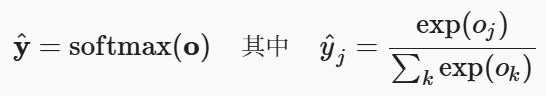
def softmax(logits):# 数值稳定版本:减去最大值max_logits = tf.reduce_max(logits, axis=-1, keepdims=True)stable_logits = logits - max_logitsexp_logits = tf.exp(stable_logits)return exp_logits / tf.reduce_sum(exp_logits, axis=-1, keepdims=True) # softmax概率tf.abs() 用于计算张量中每个元素的绝对值
tf.abs(x, name=None)- 例如,张量
[-1.0, -2.0, 3.0]使用tf.abs()函数处理它,将得到一个新的张量[1.0, 2.0, 3.0] - 在深度学习中,
tf.abs()函数通常用于计算误差(如均方误差)或用于实现某些特定的激活函数(如 ReLU)
# 1. 计算误差(L1损失)
def l1_loss(predictions, targets):"""L1损失(平均绝对误差)"""absolute_errors = tf.abs(predictions - targets)return tf.reduce_mean(absolute_errors)# 2. 梯度裁剪(基于绝对值)
def clip_gradients_by_value(gradients, clip_value):clipped_gradients = []for grad in gradients:clipped_grad = tf.clip_by_value(grad, -clip_value, clip_value)clipped_gradients.append(clipped_grad)return clipped_gradients
tf.math.rint()
tf.math.rint() 用于对输入张量中的每个元素执行 “四舍五入到最近的整数” 的操作。它的名称来源于 “round to integer” 的缩写
对称性:rint(-x) = -rint(x)
tf.math.rint(x) 将输入张量 x 中的每个元素四舍五入到最接近的整数,规则如下:
- 如果小数部分 等于 0.5,则向 最近的偶数 舍入(银行家舍入法,Bankers' Rounding)。例如
2.5→2,3.5→4 - 其他情况按 四舍五入 处理。例如
1.3→1,1.7→2
与类似函数的对比:
| 函数 | 行为 | 示例输入 [1.3, 1.5, 2.5, -1.7] |
|---|---|---|
tf.math.rint() | 四舍五入到最近整数(0.5时向偶数舍入) | [1., 2., 2., -2.] |
tf.math.round() | 四舍五入到最近整数(0.5时远离零舍入) | [1., 2., 3., -2.] |
tf.floor() | 向下取整(向负无穷方向) | [1., 1., 2., -2.] |
tf.ceil() | 向上取整(向正无穷方向) | [2., 2., 3., -1.] |
为什么用 rint 而不是 round?
rint的银行家舍入法(偶数舍入)在统计上更公平,能减少舍入偏差的累积- 例如,对
[0.5, 1.5, 2.5]取平均:rint结果[0., 2., 2.]→ 均值1.33round结果[1., 2., 3.]→ 均值2.0(偏差更大)
tf.math.log1p()
tf.math.log1p() 用于计算 log(1 + x),其中 log 是自然对数(底数是 e)
它在数值计算中比直接使用 tf.math.log(1 + x) 更加精确和稳定。比如,如果 x 是一个很小的正数(比如 1e-50),那么 1 + x 仍然接近于 1,在普通的数值精度下 log(1 + x) 可能就直接被计算为0;但如果使用 log1p 函数,就可以得到一个非零的、并且相对精确的结果
应用:pairwise_logistic_loss(完整代码参考 GitHub - tf2_pairwise_logistic_loss.py)
# 简化版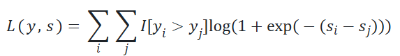
def pairwise_logistic_loss(labels,logits,temperature=1.0, # 用于缩放logitshinge_margin=None): # 正负样本对的logits最小差异# 缩放logitslogits = logits / temperature# 计算所有样本对的logits差pairwise_logits = tf.expand_dims(logits, -1) - tf.expand_dims(logits, 0)# 构建样本对掩码 (yi > yj)pairwise_mask = tf.greater(tf.expand_dims(labels, -1) - tf.expand_dims(labels, 0), 0)# hinge margin约束 (可选)if hinge_margin is not None:hinge_mask = tf.less(pairwise_logits, hinge_margin) # logits < margin 返回true,此时才需计算losspairwise_mask = tf.logical_and(pairwise_mask, hinge_mask)# 提取有效样本对pairwise_logits = tf.boolean_mask(pairwise_logits, pairwise_mask)num_pair = tf.size(pairwise_logits)# 等价于 log(1 + exp(-pairwise_logits)),通过 relu 和 log1p 实现数值稳定性losses = tf.nn.relu(-pairwise_logits) + tf.math.log1p(tf.exp(-tf.abs(pairwise_logits)))return tf.reduce_mean(losses)tf.nn.l2_normalize()
tf.nn.l2_normalize 用于对输入的张量进行 L2范数归一化处理,即输入张量的每个元素都会除以其L2范数(也就是输入张量的所有元素的平方和的平方根),使得输出张量的 L2范数为1
tf.nn.l2_normalize(x, axis=None, epsilon=1e-12, name=None)x:输入张量,希望对其进行 L2范数归一化axis:进行归一化的轴的索引。例如,如果输入是一个二维张量(也就是一个矩阵),并且希望每一行都进行归一化处理,那么应设置axis=1epsilon:一个小的浮点数,加在范数的平方上,以防止除以零
import tensorflow as tfx = tf.constant([3.0, 4.0])normalized_x = tf.nn.l2_normalize(x)
print(normalized_x)
输出结果为:
tf.Tensor([0.6 0.8], shape=(2,), dtype=float32)这是因为 x 的 L2范数是 5(根号下 3 的平方加 4 的平方),所以 x 的每个元素都除以 5,得到了新的归一化张量 normalized_x
tf.nn.relu()
tf.nn.relu() 是 "Rectified Linear Unit"(修正线性单元) 的缩写,是一个常用的激活函数
- 引入非线性:如果没有激活函数,神经网络无论有多少层都等价于一个线性模型。ReLU 提供了非线性变换,使神经网络能够学习复杂的模式
- 缓解梯度消失问题:与 sigmoid、tanh 等激活函数相比,ReLU 在正区间的梯度恒为 1,有效缓解了梯度消失问题
- 计算高效:ReLU 的计算非常简单(只是比较和取最大值),相比 sigmoid/tanh,训练收敛速度更快
数学表达式如下:ReLU(x) = max(0, x)。只要输入 x 是负数,ReLU(x) 就会返回0;若输入 x 是正数或者 0,则 ReLU(x) 就直接返回 x
# ReLU 激活函数: max(0, x)
def relu_activation(x):return tf.maximum(x, 0.0)
在神经网络中的应用:
import tensorflow as tf# 方法1:作为独立的激活函数层
model = tf.keras.Sequential([tf.keras.layers.Dense(64),  # 无激活函数的全连接层tf.keras.layers.Lambda(lambda x: tf.nn.relu(x))  # 使用 ReLU
])# 方法2:更常用的方式 - 直接在 Dense 层中指定
model = tf.keras.Sequential([tf.keras.layers.Dense(64, activation='relu'),  # 直接使用 relutf.keras.layers.Dense(32, activation='relu'),tf.keras.layers.Dense(10, activation='softmax')
])
变种:LeakyReLU
- ReLU 有 “神经元死亡” 的问题,即如果大量神经元输出为 0,可能永远无法被激活
# 标准 ReLU
output = tf.nn.relu(x)# Leaky ReLU - 负值有小的斜率,避免"神经元死亡"
output = tf.nn.leaky_relu(x, alpha=0.01)  # alpha 通常为 0.01
最佳实践:
- 在大多数网络的隐藏层中,ReLU 是默认选择;而输出层通常根据任务选择适当的激活函数(如 softmax 用于分类,linear 用于回归)
- 与批量归一化 BatchNorm 结合使用效果更好
- 使用 He 初始化(论文 https://arxiv.org/abs/1502.01852)配合 ReLU
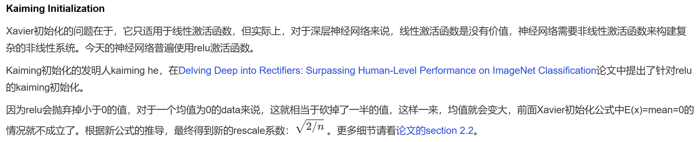
# 推荐:ReLU + He 初始化的配置
tf.keras.layers.Dense(64, activation='relu', kernel_initializer='he_normal')
tf.random.normal()
tf.random.normal() 用于生成正态分布(高斯分布)随机数
tf.random.normal(shape,                      # 输出张量的形状mean=0.0,                   # 正态分布的均值stddev=1.0,                 # 正态分布的标准差 (非负)dtype=tf.dtypes.float32,    # 输出数据类型seed=None,                  # 随机种子,用于重现结果name=None
)mean:控制分布的中心位置-
stddev:控制分布的扩散程度
设置随机种子保证可重现性,可以在调用 tf.random.normal() 之前加一行:
tf.random.set_seed(42)
应用:数据增强 - 向训练数据添加噪声
def training_fn():# 训练时的操作:添加噪声进行数据增强noise = tf.random.normal(tf.shape(input_data), stddev=0.1)return input_data + noise应用:神经网络权重初始化
def initialize_dense_layer(input_dim, output_dim, initialization='he'):"""全连接层权重初始化"""if initialization == 'he':# He初始化:适合ReLU激活函数stddev = tf.sqrt(2.0 / input_dim)elif initialization == 'xavier':# Xavier初始化:适合tanh/sigmoid激活函数stddev = tf.sqrt(1.0 / input_dim)else:stddev = 0.01weights = tf.random.normal(shape=[input_dim, output_dim],mean=0.0,stddev=stddev)biases = tf.zeros([output_dim])return weights, biasestf.expand_dims()
tf.expand_dims()用于扩展张量维度,通过在指定位置插入长度为1的新维度来改变张量的形状
tf.expand_dims(input, axis, name=None)一维张量扩展示例:
import tensorflow as tfvector = tf.constant([1, 2, 3])
print("原始张量:", vector.shape)  # (3,)# 在不同位置扩展维度
expanded_0 = tf.expand_dims(vector, axis=0)
print("axis=0:", expanded_0.shape)  # (1, 3)
# [[1, 2, 3]]expanded_1 = tf.expand_dims(vector, axis=1)
print("axis=1:", expanded_1.shape)  # (3, 1)
# [[1], [2], [3]]expanded_neg = tf.expand_dims(vector, axis=-1)
print("axis=-1:", expanded_neg.shape)  # (3, 1)
# [[1], [2], [3]]
二维张量扩展示例:
import tensorflow as tfmatrix = tf.constant([[1, 2, 3],[4, 5, 6]])
print("原始矩阵形状:", matrix.shape)  # (2, 3)# 在不同位置扩展维度
expanded_0 = tf.expand_dims(matrix, axis=0)
print("axis=0:", expanded_0.shape)  # (1, 2, 3)expanded_1 = tf.expand_dims(matrix, axis=1)
print("axis=1:", expanded_1.shape)  # (2, 1, 3)expanded_2 = tf.expand_dims(matrix, axis=2)
print("axis=2:", expanded_2.shape)  # (2, 3, 1)expanded_neg1 = tf.expand_dims(matrix, axis=-1)
print("axis=-1:", expanded_neg1.shape)  # (2, 3, 1)expanded_neg2 = tf.expand_dims(matrix, axis=-2)
print("axis=-2:", expanded_neg2.shape)  # (2, 1, 3)
在 pairwise logistic loss 中的应用:
import tensorflow as tf# 利用广播机制,生成所有样本对(i,j)的logits差。shape: [batch_size, batch_size]
pairwise_logits = tf.math.subtract(tf.expand_dims(logits, -1), tf.expand_dims(logits, 0))   # 前者[batch_size, 1],后者[1, batch_size]
# 标记所有满足 yi > yj 的样本对(i,j),返回true or false
pairwise_mask = tf.greater(tf.expand_dims(labels, -1) - tf.expand_dims(labels, 0), 0)
tf.reshape()
用于改变张量形状,可以重新排列张量的维度而不改变其数据
tf.reshape(tensor, shape, name=None)tensor:要重塑的输入张量shape:目标形状,可以是一个列表、元组或张量
import tensorflow as tfmatrix = tf.constant([[1, 2, 3],[4, 5, 6]])  # (2, 3)reshaped = tf.reshape(matrix, [3, 2])
print(reshaped.numpy())  # (3, 2)
# [[1 2]
#  [3 4]
#  [5 6]]
特殊形状值 -1 代表自动推断维度,但只能有一个 -1,否则无法确定维度
import tensorflow as tfvector = tf.constant([1, 2, 3, 4, 5, 6, 7, 8, 9, 10, 11, 12])
auto_rows = tf.reshape(vector, [-1, 3])
print(auto_rows.shape)  # (4, 3)# 当新的形状参数为 [-1] 时,意味着要将输入张量扁平化为一维张量
matrix = tf.constant([[1, 2, 3], [4, 5, 6]])  # (2, 3)
reshaped = tf.reshape(matrix, [-1])
print(reshaped)    # tf.Tensor([1 2 3 4 5 6], shape=(6,), dtype=int32)
应用:多头注意力
import tensorflow as tfdef multi_head_attention_reshape(Q, num_heads):batch_size = tf.shape(Q)[0]seq_length = tf.shape(Q)[1]depth = tf.shape(Q)[2]# 重塑为 (batch_size, seq_length, num_heads, depth_per_head)depth_per_head = depth // num_headsreshaped_Q = tf.reshape(Q, [batch_size, seq_length, num_heads, depth_per_head])# 转置为 (batch_size, num_heads, seq_length, depth_per_head)transposed_Q = tf.transpose(reshaped_Q, [0, 2, 1, 3])return transposed_Q# 示例
Q = tf.random.normal([2, 5, 64])  # (batch, seq_len, depth)
num_heads = 8
multi_head_Q = multi_head_attention_reshape(Q, num_heads)
print("原始Q形状:", Q.shape)          # (2, 5, 64)
print("多头Q形状:", multi_head_Q.shape)  # (2, 8, 5, 8)
tf.range()
tf.range 用于创建一个包含等差数列的一维张量,类似于 Python 内置的 range() 函数,但返回的是 TensorFlow 张量
tf.range(start, limit=None, delta=1, dtype=None, name=None)- start:序列的起始值(包含)
- limit:序列的结束值(不包含)
- delta:步长,默认为 1,可以为负数
- dtype:输出张量的数据类型
import tensorflow as tfindices = tf.range(5)
print(indices)
输出结果为:
tf.Tensor([0 1 2 3 4], shape=(5,), dtype=int32)应用:Transformer模型中的位置编码(提供序列中每个位置的位置信息)
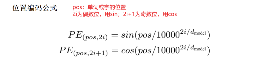
def positional_encoding(sequence_length, d_model):# [:, tf.newaxis]:增加一个维度,从 (seq_len,) 变为 (seq_len, 1) 的列向量position = tf.range(sequence_length, dtype=tf.float32)[:, tf.newaxis] # (seq_len, 1)div_term = tf.exp(tf.range(0, d_model, 2, dtype=tf.float32) * # 偶数索引-(tf.math.log(10000.0) / d_model))# 原公式:exp(2i * (-ln(10000)/d_model))# = exp(-2i * ln(10000)/d_model)# = (exp(ln(10000)))^(-2i/d_model)# = 10000^(-2i/d_model)angle_rates = position * div_term # (seq_len, d_model/2)sin_encoding = tf.sin(angle_rates) # 偶数列 - 正弦函数cos_encoding = tf.cos(angle_rates) # 奇数列 - 余弦函数# 交错拼接正弦和余弦positional_encoding = tf.stack([sin_encoding, cos_encoding], axis=2) # (seq_len, d_model/2, 2)positional_encoding = tf.reshape(positional_encoding, [sequence_length, d_model]) # (seq_len, d_model)return positional_encoding应用:创建 one-hot 编码
num_classes = 5
labels = tf.constant([0, 2, 4])class_range = tf.range(num_classes)
print(class_range.numpy())  # [0 1 2 3 4]# 创建 one-hot 编码
one_hot = tf.cast(tf.equal(labels[:, tf.newaxis], class_range), tf.float32)
print(one_hot.numpy())
# [[1. 0. 0. 0. 0.]
#  [0. 0. 1. 0. 0.]
#  [0. 0. 0. 0. 1.]]
tf.sequence_mask()
tf.sequence_mask() 用于创建序列掩码,根据序列长度生成布尔掩码,常用于处理变长序列数据
tf.sequence_mask(lengths, maxlen=None, dtype=tf.dtypes.bool, name=None)lengths:序列长度张量,1D 整数张量。输入形状为[batch_size]maxlen:最大序列长度,如果不指定则使用lengths中的最大值dtype:输出掩码的数据类型,默认为tf.bool,也可以为tf.int32/tf.float32-
输出掩码形状为
[batch_size, maxlen]
import tensorflow as tf# 创建序列长度掩码
sequence_lengths = tf.constant([3, 5, 2, 4])
mask = tf.sequence_mask(sequence_lengths, 5)
print(mask.numpy())# [[ True  True  True False False]
#  [ True  True  True  True  True]
#  [ True  True False False False]
# [ True True True True False]]应用:获取序列的实际长度 -> 创建掩码 -> 在模型计算中应用掩码 -> 在损失计算中忽略填充位置
import tensorflow as tf# 序列的实际长度
sequence_lengths = tf.constant([2, 4, 3])# 创建掩码
mask = tf.sequence_mask(sequence_lengths, maxlen=5)    # shape=(3, 5)# 在模型计算中应用掩码
lstm_output = tf.random.normal([3, 5, 8])  # 模拟LSTM输出 (batch_size, seq_len, hidden_size)
mask_float = tf.cast(mask, tf.float32)[:, :, tf.newaxis]   # (3, 5, 1)
masked_output = lstm_output * mask_float   # (3, 5, 8)# 在损失计算中忽略填充位置
# 真实标签
true_labels = tf.constant([[10, 20, 0, 0, 0],[30, 40, 50, 60, 0], [70, 80, 90, 0, 0]
])# 预测标签
pred_labels = tf.constant([[12, 18, 5, 8, 3],[28, 42, 48, 65, 2],[72, 78, 85, 4, 1]
])# 计算MSE损失(只计算有效位置)
mse = tf.square(true_labels - pred_labels)
masked_mse = mse * tf.cast(mask, tf.float32)
# 只对有效位置求平均
valid_positions = tf.reduce_sum(tf.cast(mask, tf.float32))
total_loss = tf.reduce_sum(masked_mse) / valid_positions
输出结果为:
# mse
tf.Tensor(
[[ 4  4 25 64  9][ 4  4  4 25  4][ 4  4 25 16  1]], shape=(3, 5), dtype=int32)# masked_mse
tf.Tensor(
[[ 4  4  0  0  0][ 4  4  4 25  0][ 4  4 25  0  0]], shape=(3, 5), dtype=int32)# valid_positions
tf.Tensor(9, shape=(), dtype=int32)# total_loss
tf.Tensor(8.666666666666666, shape=(), dtype=float64)
相关函数:
- 结合
tf.boolean_mask()提取有效元素 - 使用
tf.where()应用掩码,即根据条件选择元素
tf.nn.embedding_lookup()
tf.nn.embedding_lookup() 用于词嵌入查找,它根据索引从嵌入矩阵中查找对应的嵌入向量
tf.nn.embedding_lookup(params, ids, max_norm=None, name=None)params:嵌入矩阵,形状为[vocab_size, embedding_dim]ids:要查找的索引,可以是标量、向量或更高维度的张量max_norm:如果提供,会对查找的嵌入向量进行 L2归一化- 输出形状为
ids.shape + [embedding_dim]
如:params 是一个形状为 [vocab_size, embedding_dim] 的词嵌入矩阵,ids 是一个形状为[batch_size, sequence_length] 的整数张量,那么这个操作将会返回一个形状为 [batch_size, sequence_length, embedding_dim] 的向量。这个向量就是每个ID在词嵌入矩阵中对应的向量
其他常用
class、__init__、call
Python用法,非Tensorflow
在 Python 中,当我们定义一个类时,通常会用到 __init__ 和 call 这两个特殊的方法
__init__方法:此方法在 Python 中被称为初始化方法或构造器方法。当一个类被实例化(即创建一个类的对象)时,就会自动调用这个方法。通常在__init__方法中定义那些在对象创建时就需要被初始化的属性call方法:此方法在 Python 中被称为可调用方法。当一个对象像函数那样被使用时,就会自动触发call方法
例如,我们定义一个名为 Model 的类,并使用 __init__ 方法为其初始化一个属性(name 是在创建 Model 类的对象时需要传入的参数);同时可以为上述的 Model 类添加一个 call 方法(可以像调用函数一样调用 Model 类的对象,并向其传递参数 x)
class Model:def __init__(self, name):self.name = namedef __call__(self, x):return f'Model {self.name} process {x}'这两个方法可以帮我们理解在类中需要哪些输入参数。在 __init__ 方法中定义的是在对象创建时需要的输入,而在 __call__ 方法中定义的是在对象被函数式调用时需要的输入
# 使用上述的 Model 类为例
model = Model('Example')  # 创建对象时,需要一个名为 `name` 的输入
output = model('input')   # 对象被函数式调用时,需要一个名为 `x` 的输入
assign_sub / assign
assign_sub 用于对变量的值进行就地(in-place)减法操作,即将变量的值减去指定的值,并将结果重新赋值给该变量。通常用于优化算法中更新模型参数(如权重)或优化器中的状态变量
tf.Variable.assign_sub(value)value:要减去的值,可以是一个标量、张量或与变量形状相同的张量- 返回更新后的变量
特点:
- 就地操作:
assign_sub会直接修改变量的值,而不是创建一个新的变量 - 仅适用于变量:
assign_sub只能用于tf.Variable类型的对象,不能用于普通的张量(tf.Tensor) - 自动类型转换:如果
value的类型与变量的类型不同,会自动进行类型转换
import tensorflow as tf# 创建一个变量
x = tf.Variable(10.0)# 使用 assign_sub 减去一个值
x.assign_sub(3.0)
print("Updated x:", x.numpy()) # 7.0在训练神经网络时,assign_sub 通常用于更新模型参数。例如,在使用梯度下降法时,可以用 assign_sub 来更新权重:
import tensorflow as tf# 创建一个变量(模拟权重)
weight = tf.Variable(5.0)
# 模拟梯度
gradient = 2.0
# 学习率
learning_rate = 0.1# 更新权重:weight = weight - learning_rate * gradient
weight.assign_sub(learning_rate * gradient)
print("Updated weight:", weight.numpy())   # 4.8
assign_sub 是对变量进行减法操作,而 assign 是直接为变量赋值,例如:
x.assign(7.0) # 将 x 的值设置为 7.0
tf.float32.min
tf.float32.min 是 TensorFlow 的一个标量,表示 float32 数据类型能够表示的最小正数。常作为数值稳定性的阈值,用于下溢保护
def stable_softmax(logits):"""数值稳定的 softmax"""# 减去最大值提高数值稳定性max_logits = tf.reduce_max(logits, axis=-1, keepdims=True)stable_logits = logits - max_logits# 计算指数exp_logits = tf.exp(stable_logits)# 保护下溢exp_logits = tf.maximum(exp_logits, tf.float32.min)# 归一化return exp_logits / tf.reduce_sum(exp_logits, axis=-1, keepdims=True)logging.info()
Python用法,非Tensorflow
Python logging 模块定义了多个日志级别(按严重程度递增):
| 级别 | 数值 | 函数 | 用途 |
|---|---|---|---|
| DEBUG | 10 | logging.debug() | 详细的调试信息 |
| INFO | 20 | logging.info() | 确认程序按预期运行 |
| WARNING | 30 | logging.warning() | 表示意外情况,但程序仍能运行 |
| ERROR | 40 | logging.error() | 由于严重问题,程序无法执行某些功能 |
| CRITICAL | 50 | logging.critical() | 严重错误,程序本身可能无法继续运行 |
logging.info() 的级别为 20,通常用于记录程序正常运行时的关键信息。注意,默认的日志级别是 WARNING(30)才会输出:
import logging# 设置日志级别为 INFO
logging.basicConfig(level=logging.INFO)logging.info("程序启动")
logging.debug("这条调试消息不会显示")  # 因为级别低于 INFO
logging.warning("这是一条警告消息")    # 这会显示
完整配置:
import logginglogging.basicConfig(level=logging.INFO,# %(asctime)s - 时间戳# %(name)s - 记录器名称# %(levelname)s - 日志级别# %(message)s - 日志消息format='%(asctime)s - %(name)s - %(levelname)s - %(message)s',datefmt='%Y-%m-%d %H:%M:%S',filename='app.log',  # 可选:输出到文件filemode='a'         # 可选:追加模式
)-
print()只是临时调试,logging.info()提供完整的日志管理
在深度学习模型中的应用:
import logging
import tensorflow as tfdef train_model():logging.basicConfig(level=logging.INFO,format='%(asctime)s - %(levelname)s - %(message)s')logging.info("开始模型训练")# 加载数据logging.info("加载训练数据")(x_train, y_train), (x_test, y_test) = tf.keras.datasets.mnist.load_data()logging.info(f"训练数据形状: {x_train.shape}")# 构建模型logging.info("构建神经网络模型")model = tf.keras.Sequential([tf.keras.layers.Flatten(input_shape=(28, 28)),tf.keras.layers.Dense(128, activation='relu'),tf.keras.layers.Dense(10)])# 编译模型logging.info("编译模型")model.compile(optimizer='adam',loss=tf.keras.losses.SparseCategoricalCrossentropy(from_logits=True),metrics=['accuracy'])# 训练模型logging.info("开始训练循环")model.fit(x_train, y_train, epochs=5, verbose=0)logging.info("模型训练完成")# 评估模型logging.info("评估模型性能")test_loss, test_acc = model.evaluate(x_test, y_test, verbose=0)logging.info(f"测试准确率: {test_acc:.4f}")train_model()