当前位置：首页 > news >正文

糖尿病预测多个机器学习维度预测

news 2025/11/4 8:18:46

资料来源

1. 简介
- 问题陈述
- 数据描述
2. 导入库
3. 基础探索
- 读取数据集
- 基本信息
- 数据可视化
4. 数据预处理
5. 机器学习模型
- 逻辑回归
- 随机森林分类器
- 随机森林超参数调优
- 决策树分类器
- 决策树超参数调优
- K近邻分类器模型
- KNN超参数调优
- 支持向量分类器
- AdaBoost分类器
- 梯度提升分类器
- XGBoost分类器
6. 结论
- 总结
- 未来可能的工作
7. 作者寄语

1 | 简介

1.1 | 问题陈述

该数据集的目标是构建一个预测模型，用于诊断至少21岁且具有皮马印第安血统的女性患者是否患有糖尿病。该模型应根据多项诊断指标预测患者是否患有糖尿病（结果=1）或未患糖尿病（结果=0），这些指标包括葡萄糖水平、血压、皮肤厚度、胰岛素水平、BMI、糖尿病谱系功能和年龄。

1.2 | 数据描述

编号	列名	含义
1	Pregnancies	怀孕次数
2	Glucose	血糖葡萄糖水平
3	BloodPressure	血压测量值
4	SkinThickness	皮肤厚度
5	Insulin	血液胰岛素水平
6	BMI	身体质量指数
7	DiabetesPedigreeFunction	糖尿病遗传概率
8	Age	年龄
9	Outcome	最终结果 (1: 患有糖尿病; 0: 未患糖尿病)

2 | 导入库

#导包
import pandas as pd
import numpy as np
import matplotlib.pyplot as plt
%matplotlib inline
import seaborn as sns
from sklearn.model_selection import GridSearchCV, cross_val_score
from sklearn.preprocessing import StandardScaler
from sklearn.ensemble import RandomForestClassifier, VotingClassifier
from sklearn.tree import DecisionTreeClassifier
from sklearn.svm import SVC
from sklearn.neighbors import KNeighborsClassifier
from sklearn.linear_model import LogisticRegression
from xgboost import XGBClassifier
from lightgbm import LGBMClassifier
from sklearn.ensemble import AdaBoostClassifier, GradientBoostingClassifier
import joblib
import warnings
warnings.filterwarnings('ignore')

3 | 基础探索

3.1 | 读取数据集

df = pd.read_csv('diabetes.csv')

3.2 | 基础信息

3.2.1 | 显示数据内容

styled_df = df.head(5).style# 设置整个DataFrame的背景颜色、文字颜色和边框
styled_df.set_properties(**{"background-color": "#254E58", "color": "#e9c46a", "border": "1.5px solid black"})# 修改表头(th)的颜色和背景颜色
styled_df.set_table_styles([{"selector": "th", "props": [("color", 'white'), ("background-color", "#333333")]}
])

3.2.2 | 行数与列数

rows , col =  df.shape
print(f"行数 : {rows} \n列数 : {col}")

输出:

行数 : 768 
列数 : 9

3.2.3 | 基本信息

df.info()

输出:

<class 'pandas.core.frame.DataFrame'>
RangeIndex: 768 entries, 0 to 767
Data columns (total 9 columns):#   Column                    Non-Null Count  Dtype  
---  ------                    --------------  -----  0   Pregnancies               768 non-null    int64  1   Glucose                   768 non-null    int64  2   BloodPressure             768 non-null    int64  3   SkinThickness             768 non-null    int64  4   Insulin                   768 non-null    float645   BMI                       768 non-null    float646   DiabetesPedigreeFunction  768 non-null    float647   Age                       768 non-null    int64  8   Outcome                   768 non-null    int64  
dtypes: float64(3), int64(6)
memory usage: 54.1 KB

3.2.4 | 统计空值/缺失值

df.isnull().sum()

结果:

Pregnancies                 0
Glucose                     0
BloodPressure               0
SkinThickness               0
Insulin                     0
BMI                         0
DiabetesPedigreeFunction    0
Age                         0
Outcome                     0
dtype: int64

未发现缺失值

3.2.5 | 数据描述

styled_df = df.describe().style \.set_table_styles([{'selector': 'th', 'props': [('background-color', '#254E58'), ('color', 'white'), ('font-weight', 'bold'), ('text-align', 'left'), ('padding', '8px')]},{'selector': 'td', 'props': [('padding', '8px')]}]) \.set_properties(**{'font-size': '14px', 'background-color': '#F5F5F5', 'border-collapse': 'collapse', 'margin': '10px'})# Display the styled DataFrame
styled_df

import missingno as msnonum_columns = len(df.columns)
colors = plt.cm.viridis(np.linspace(0, 1, num_columns))  msno.bar(df, color=colors)
plt.show()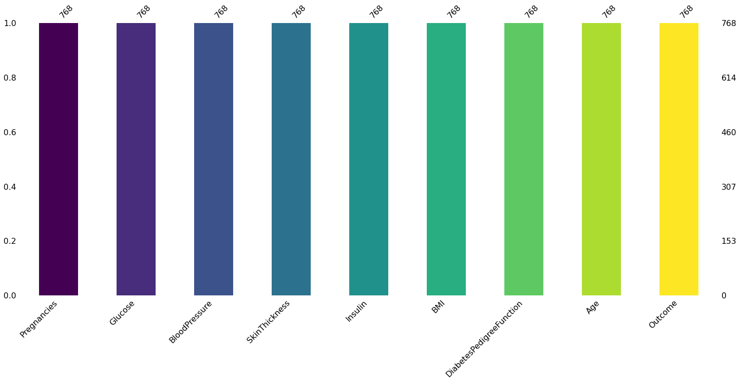

在这里插入图片描述

3.3 | 数据可视化

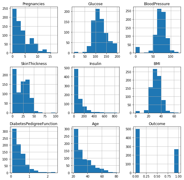
3.3.1 | 属性分布

df.hist(figsize = (10,10))
plt.show()

在这里插入图片描述

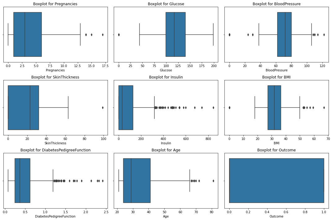
3.3.2 | 箱线图

num_rows, num_cols = 3, 3# Create subplots
fig, axes = plt.subplots(num_rows, num_cols, figsize=(15, 10))# Flatten the axes for easier iteration
axes = axes.flatten()# Loop through numeric columns and create boxplots
for i, column in enumerate(df.columns):sns.boxplot(data=df, x=column, ax=axes[i])axes[i].set_title(f'Boxplot for {column}')# Remove any remaining empty subplots
for j in range(len(df.columns), len(axes)):fig.delaxes(axes[j])# Adjust layout
plt.tight_layout()
plt.show()

在这里插入图片描述

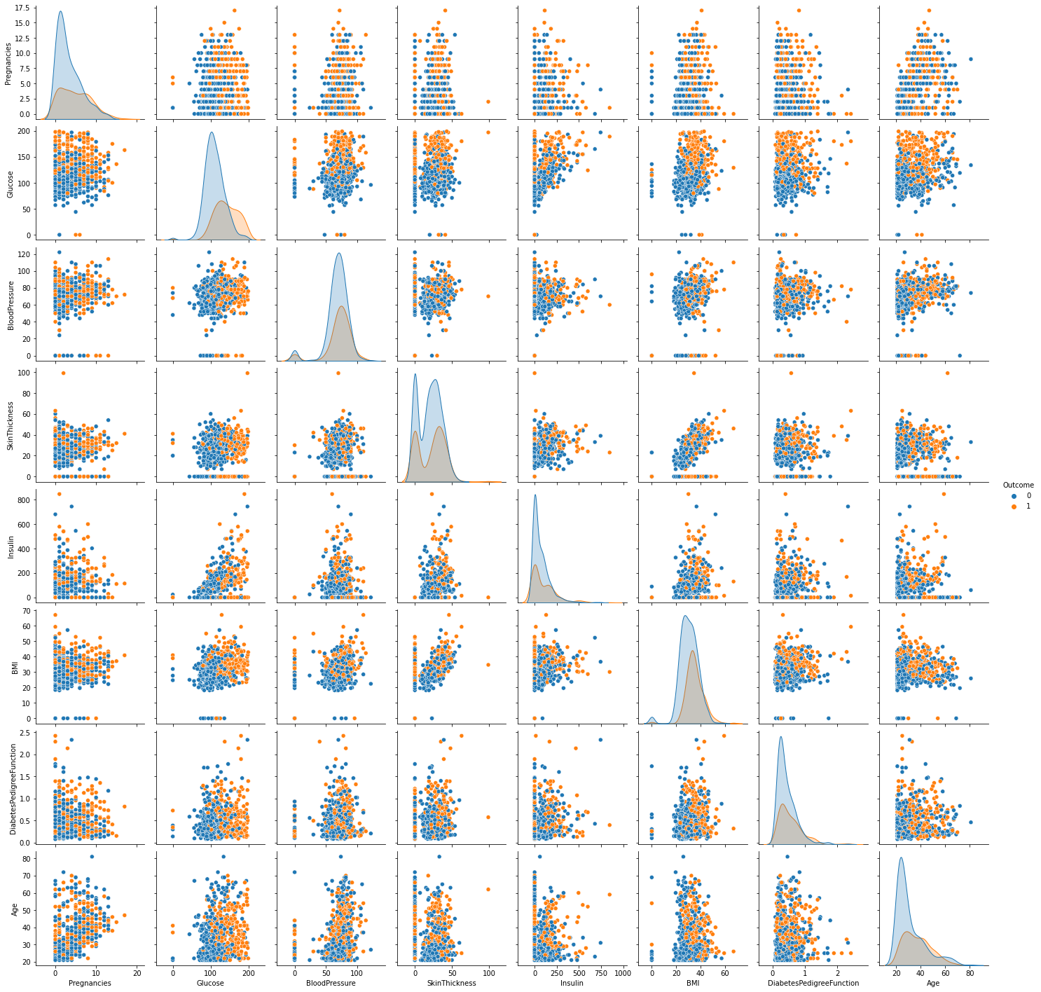
3.3.3 | 属性配对图

sns.pairplot(data = df, hue = 'Outcome' )
plt.show()

在这里插入图片描述

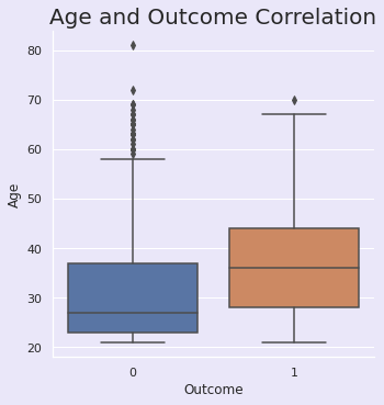
3.3.4 | 年龄与结果

sns.set(rc={"axes.facecolor":"#EAE7F9","figure.facecolor":"#EAE7F9"})
p=sns.catplot(x="Outcome",y="Age", data=df, kind='box')
plt.title("Age and Outcome Correlation", size=20, y=1.0);

在这里插入图片描述

3.3.5 | Glucose and Outcome Correlation

sns.set(rc={"axes.facecolor":"#EAE7F9","figure.facecolor":"#EAE7F9"})
p=sns.catplot(x="Outcome",y="Glucose", data=df, kind='box')
plt.title("Glucose and Outcome Correlation", size=20, y=1.0);

在这里插入图片描述

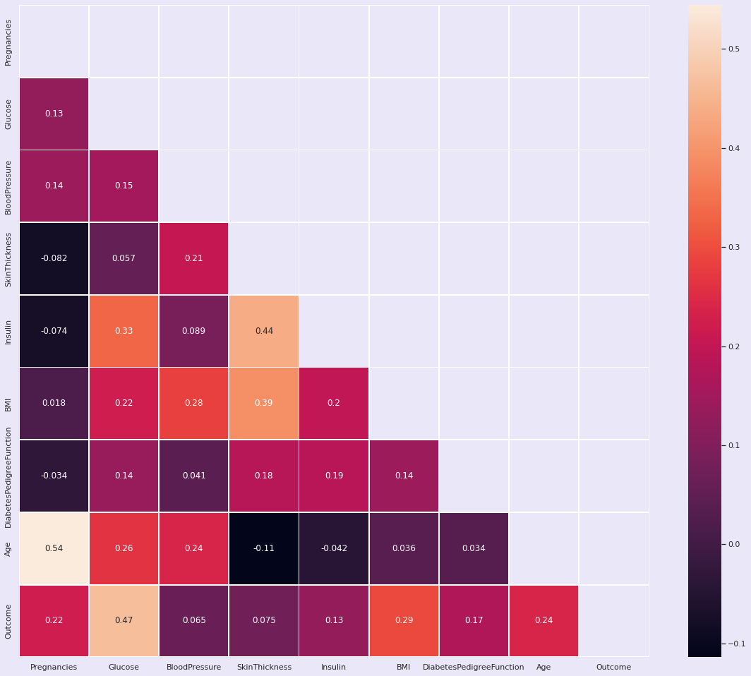
3.3.6 | 属性间相关性

plt.figure(figsize=(20, 17))
matrix = np.triu(df.corr())
sns.heatmap(df.corr(), annot=True, linewidth=.8, mask=matrix, cmap="rocket");

在这里插入图片描述

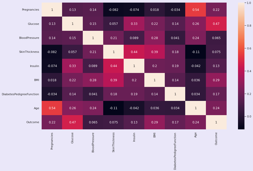
plt.figure(figsize=(16,9))
sns.heatmap(df.corr(), annot=True);

在这里插入图片描述

hig_corr = df.corr()
hig_corr_features = hig_corr.index[abs(hig_corr["Outcome"]) >= 0.2]
hig_corr_features

结果:

Index(['Pregnancies', 'Glucose', 'BMI', 'Age', 'Outcome'], dtype='object')

3.3.7 | 标准差

#Standard Deviation
df.var()

结果:

Pregnancies                    11.354056
Glucose                      1022.248314
BloodPressure                 374.647271
SkinThickness                 254.473245
Insulin                     13281.180078
BMI                            62.159984
DiabetesPedigreeFunction        0.109779
Age                           138.303046
Outcome                         0.227483
dtype: float64

4 | 数据预处理

处理异常值

numeric_columns = ['Insulin', 'DiabetesPedigreeFunction',]for column_name in numeric_columns:Q1 = np.percentile(df[column_name], 25, interpolation='midpoint')Q3 = np.percentile(df[column_name], 75, interpolation='midpoint')IQR = Q3 - Q1low_lim = Q1 - 1.5 * IQRup_lim = Q3 + 1.5 * IQR# Find outliers in the specified columnoutliers = df[(df[column_name] < low_lim) | (df[column_name] > up_lim)][column_name]# Replace outliers with the respective lower or upper limitdf[column_name] = np.where(df[column_name] < low_lim, low_lim, df[column_name])df[column_name] = np.where(df[column_name] > up_lim, up_lim, df[column_name])

获取输入和目标列

X = df.drop('Outcome', axis = 1)
y = df['Outcome']

划分训练数据

from sklearn.model_selection import train_test_splitX_train, X_test, y_train, y_test = train_test_split(X,y, test_size = 0.20)

5 | 机器学习模型

5.1 | 逻辑回归

from sklearn.linear_model import LogisticRegression
log_reg = LogisticRegression(C=1, penalty='l2', solver='liblinear', max_iter=200)
log_reg.fit(X_train, y_train)

结果:

LogisticRegression(C=1, max_iter=200, solver='liblinear')

from sklearn.metrics import confusion_matrix, accuracy_score
import matplotlib.pyplot as plt
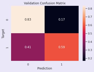
import seaborn as snsdef predict_and_plot(model, inputs, targets, name=''):preds = model.predict(inputs)accuracy = accuracy_score(targets, preds)print("Accuracy: {:.2f}%".format(accuracy * 100))cf = confusion_matrix(targets, preds, normalize='true')plt.figure()sns.heatmap(cf, annot=True)plt.xlabel('Prediction')plt.ylabel('Target')plt.title('{} Confusion Matrix'.format(name))return preds# Predict and plot on the training data
train_preds = predict_and_plot(log_reg, X_train, y_train, 'Train')# Predict and plot on the validation data
val_preds = predict_and_plot(log_reg, X_test, y_test, 'Validation')

输出:

Accuracy: 78.18%
Accuracy: 75.32%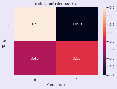

在这里插入图片描述

评估：逻辑回归模型
训练准确率 - 77.54%
验证准确率 - 77.68%

5.2 | 随机森林

from sklearn.ensemble import RandomForestClassifier
model_2 = RandomForestClassifier(n_jobs =-1, random_state = 42)
model_2.fit(X_train,y_train)

结果:

RandomForestClassifier(n_jobs=-1, random_state=42)

model_2.score(X_train,y_train)

结果:

1.0

def predict_and_plot(model, inputs,targets, name = ''):preds = model.predict(inputs)accuracy = accuracy_score(targets, preds)print("Accuracy: {:.2f}%".format(accuracy*100))cf = confusion_matrix(targets, preds, normalize = 'true')plt.figure()sns.heatmap(cf, annot = True)plt.xlabel('Prediction')plt.ylabel('Target')plt.title('{} Confusion Matrix'. format(name))return predstrain_preds = predict_and_plot(model_2, X_train, y_train, 'Train')# Predict and plot on the validation data
val_preds = predict_and_plot(model_2, X_test, y_test, 'Validation')

输出:

Accuracy: 100.00%
Accuracy: 74.03%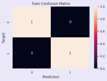

在这里插入图片描述

评估：随机森林模型：调优前
训练准确率 - 96.00%
验证准确率 - 78.08%
该模型似乎存在过拟合，因为训练准确率很高而验证准确率相对较低。

随机森林超参数调优

from sklearn.ensemble import RandomForestClassifier
from sklearn.model_selection import GridSearchCV
from sklearn.ensemble import RandomForestClassifier
from sklearn.metrics import accuracy_scoreparam_grid = {'n_estimators': [10, 20, 30],  # Adjust the number of trees in the forest'max_depth': [10, 20, 30],  # Adjust the maximum depth of each tree'min_samples_split': [2, 5, 10, 15, 20],  # Adjust the minimum samples required to split a node'min_samples_leaf': [1, 2, 4, 6, 8]  # Adjust the minimum samples required in a leaf node
}model = RandomForestClassifier(random_state=42, n_jobs=-1)
grid_search = GridSearchCV(model, param_grid, cv=5, n_jobs=-1, scoring='accuracy')
grid_search.fit(X_train, y_train)
best_model = grid_search.best_estimator_best_model.fit(X_train, y_train)# Evaluate the model on the training and validation data
train_accuracy = best_model.score(X_train, y_train)
val_accuracy = best_model.score(X_test, y_test)# Print the results
print("Training Accuracy:", train_accuracy)
print("Validation Accuracy:", val_accuracy)

输出:

Training Accuracy: 89.2%
Validation Accuracy: 87.6%

评估：超参数调优后的随机森林模型
训练准确率 - 89.2%
验证准确率 - 87.6%
与初始模型相比，过拟合现象有所减少，且准确率得到了提升。

5.4 | 决策树

from sklearn.tree import DecisionTreeClassifier
from sklearn.metrics import accuracy_scoredecision_tree_model = DecisionTreeClassifier(random_state=42)decision_tree_model.fit(X_train, y_train)train_accuracy = decision_tree_model.score(X_train, y_train)
val_accuracy = decision_tree_model.score(X_test, y_test)print("Training Accuracy:", train_accuracy)
print("Validation Accuracy:", val_accuracy)

输出:

Training Accuracy: 1.0
Validation Accuracy: 0.9415584415584416

评估：决策树模型：调优前
训练准确率 - 100%
验证准确率 - 75.0%
决策树模型对训练数据存在过拟合，在训练数据上达到了完美准确率，但在验证数据上准确率较低。

决策树超参数调优

from sklearn.tree import DecisionTreeClassifier
from sklearn.model_selection import GridSearchCVparam_grid = {'max_depth': [None, 5, 10, 15, 20],'min_samples_split': [2, 5, 10, 15, 20, 25],'min_samples_leaf': [1, 3, 5, 7],'criterion': ['gini', 'entropy']  # Add criterion hyperparameter
}decision_tree_model = DecisionTreeClassifier(random_state=42)grid_search = GridSearchCV(decision_tree_model, param_grid, cv=5, n_jobs=-1, scoring='accuracy')
grid_search.fit(X_train, y_train)best_model = grid_search.best_estimator_best_model.fit(X_train, y_train)train_accuracy = best_model.score(X_train, y_train)
val_accuracy = best_model.score(X_test, y_test)print("Training Accuracy:", train_accuracy)
print("Validation Accuracy:", val_accuracy)

评估：决策树模型
训练准确率 - 82.2%
验证准确率 - 85.5%
与初始模型相比，过拟合现象有所减少，且结果得到了改善。

5.6 | K近邻分类器模型

from sklearn.neighbors import KNeighborsClassifier
from sklearn.model_selection import train_test_split
from sklearn.metrics import accuracy_score, confusion_matrixX_train, X_val, y_train, y_val = train_test_split(X, y, test_size=0.2, random_state=42)knn_model = KNeighborsClassifier(n_neighbors=5)knn_model.fit(X_train, y_train)y_train_pred = knn_model.predict(X_train)y_val_pred = knn_model.predict(X_val)train_accuracy = accuracy_score(y_train, y_train_pred)
val_accuracy = accuracy_score(y_val, y_val_pred)print("Training Accuracy:", train_accuracy)
print("Validation Accuracy:", val_accuracy)confusion = confusion_matrix(y_val, y_val_pred)plt.figure(figsize=(6, 4))
sns.heatmap(confusion, annot=True, fmt='d', cmap='Blues', cbar=False)
plt.xlabel('Predicted')
plt.ylabel('Actual')
plt.title('Confusion Matrix (Validation)')
plt.show()

输出:

Training Accuracy: 0.8045602605863192
Validation Accuracy: 0.6688311688311688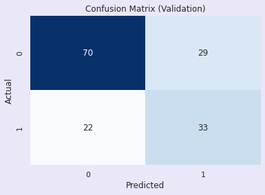

在这里插入图片描述

评估：K近邻分类器：调优前
训练准确率 - 80.0%
验证准确率 - 66.00%

KNN超参数调优

from sklearn.neighbors import KNeighborsClassifier
from sklearn.model_selection import GridSearchCV
from sklearn.metrics import accuracy_scoreparam_grid = {'n_neighbors': [1, 3, 5, 7, 9]  # Adjust the number of neighbors to explore
}knn_model = KNeighborsClassifier()grid_search = GridSearchCV(knn_model, param_grid, cv=5, scoring='accuracy')
grid_search.fit(X_train, y_train)best_model = grid_search.best_estimator_y_train_pred = best_model.predict(X_train)y_val_pred = best_model.predict(X_val)train_accuracy = accuracy_score(y_train, y_train_pred)
val_accuracy = accuracy_score(y_val, y_val_pred)print("Training Accuracy with Best Hyperparameters:", train_accuracy)
print("Validation Accuracy with Best Hyperparameters:", val_accuracy)

输出:

Training Accuracy with Best Hyperparameters: 0.7947882736156352
Validation Accuracy with Best Hyperparameters: 0.7272727272727273

评估：调优后的KNN模型
训练准确率 - 79.4%
验证准确率 - 72.7%

5.8 | 支持向量分类器

X_train, X_val, y_train, y_val = train_test_split(X, y, test_size=0.2, random_state=42)svm_model = SVC(kernel='linear')svm_model.fit(X_train, y_train)y_train_pred = svm_model.predict(X_train)y_val_pred = svm_model.predict(X_val)train_accuracy = accuracy_score(y_train, y_train_pred)val_accuracy = accuracy_score(y_val, y_val_pred)print("Training Accuracy:", train_accuracy)
print("Validation Accuracy:", val_accuracy)train_confusion = confusion_matrix(y_train, y_train_pred)
val_confusion = confusion_matrix(y_val, y_val_pred)plt.figure(figsize=(12, 5))
plt.subplot(1, 2, 1)
sns.heatmap(train_confusion, annot=True, fmt='d', cmap='Blues', cbar=False)
plt.xlabel('Predicted')
plt.ylabel('Actual')
plt.title('Confusion Matrix (Training)')plt.subplot(1, 2, 2)
sns.heatmap(val_confusion, annot=True, fmt='d', cmap='Blues', cbar=False)
plt.xlabel('Predicted')
plt.ylabel('Actual')
plt.title('Confusion Matrix (Validation)')
plt.show()

输出:

Training Accuracy: 0.7785016286644951
Validation Accuracy: 0.7727272727272727

在这里插入图片描述

评估：支持向量分类器
训练准确率 - 77.8%
验证准确率 - 77.2%

5.9 | AdaBoost分类器

from sklearn.ensemble import AdaBoostClassifier
from sklearn.metrics import accuracy_score, confusion_matrixadaboost_model = AdaBoostClassifier(n_estimators=50, random_state=42)adaboost_model.fit(X_train, y_train)y_train_pred_adaboost = adaboost_model.predict(X_train)y_val_pred_adaboost = adaboost_model.predict(X_val)train_accuracy_adaboost = accuracy_score(y_train, y_train_pred_adaboost)val_accuracy_adaboost = accuracy_score(y_val, y_val_pred_adaboost)print("AdaBoost Training Accuracy:", train_accuracy_adaboost)
print("AdaBoost Validation Accuracy:", val_accuracy_adaboost)confusion_adaboost = confusion_matrix(y_val, y_val_pred_adaboost)# Plot the confusion matrix
plt.figure()
sns.heatmap(confusion_adaboost, annot=True, fmt='d', cmap='Blues', cbar=False)
plt.xlabel('Predicted')
plt.ylabel('Actual')
plt.title('AdaBoost Confusion Matrix (Validation)')
plt.show()

输出:

AdaBoost Training Accuracy: 0.8224755700325733
AdaBoost Validation Accuracy: 0.7402597402597403

在这里插入图片描述

评估：AdaBoost分类器
训练准确率 - 82.4%
验证准确率 - 74.0%

5.7 | Gradient Boosting Classifier

from sklearn.ensemble import GradientBoostingClassifier# 创建梯度提升分类器
gbm_model = GradientBoostingClassifier(n_estimators=100, max_depth=3, random_state=42)# 将GBM模型拟合到训练数据
gbm_model.fit(X_train, y_train)# 对训练数据进行预测
y_train_pred_gbm = gbm_model.predict(X_train)# 对验证数据进行预测
y_val_pred_gbm = gbm_model.predict(X_val)# 计算训练准确率
train_accuracy_gbm = accuracy_score(y_train, y_train_pred_gbm)# 计算验证准确率
val_accuracy_gbm = accuracy_score(y_val, y_val_pred_gbm)# 打印训练和验证准确率
print("GBM训练准确率:", train_accuracy_gbm)
print("GBM验证准确率:", val_accuracy_gbm)

输出:

GBM Training Accuracy: 0.9429967426710097
GBM Validation Accuracy: 0.7532467532467533

评估：梯度提升分类器
训练准确率 - 94.2%
验证准确率 - 75.3%

5.11 | XGBoost分类器

from xgboost import XGBClassifier# Create an XGBoost classifier
xgboost_model = XGBClassifier(n_estimators=100, max_depth=3, random_state=42)# Fit the XGBoost model to the training data
xgboost_model.fit(X_train, y_train)# Make predictions on the training data
y_train_pred_xgboost = xgboost_model.predict(X_train)# Make predictions on the validation data
y_val_pred_xgboost = xgboost_model.predict(X_val)# Calculate the training accuracy
train_accuracy_xgboost = accuracy_score(y_train, y_train_pred_xgboost)# Calculate the validation accuracy
val_accuracy_xgboost = accuracy_score(y_val, y_val_pred_xgboost)# Print the training and validation accuracies
print("XGBoost Training Accuracy:", train_accuracy_xgboost)
print("XGBoost Validation Accuracy:", val_accuracy_xgboost)

输出:

[14:40:09] WARNING: ../src/learner.cc:1115: Starting in XGBoost 1.3.0, the default evaluation metric used with the objective 'binary:logistic' was changed from 'error' to 'logloss'. Explicitly set eval_metric if you'd like to restore the old behavior.
XGBoost Training Accuracy: 0.988599348534202
XGBoost Validation Accuracy: 0.7272727272727273

评估：XGBoost分类器
训练准确率 - 98.4%
验证准确率 - 72.7%