Lambert W 函数简要探讨
注:本文为 “Lambert W” 英文引文,机翻未校。
如有内容异常,请看原文。
A Brief Look into the Lambert W Function
对朗伯 W 函数的简要探讨
Thomas P. Dence
Ashland University, Ashland, USA
Email: tdence@ashland.edu
Received December 4, 2012; revised March 14, 2013; accepted March 22, 2013
Copyright © 2013 Thomas P. Dence. This is an open access article distributed under the Creative Commons Attribution License, which permits unrestricted use, distribution, and reproduction in any medium, provided the original work is properly cited.
ABSTRACT
摘要
The Lambert W function has its origin traced back 250 years, but it’s just been in the past several decades when some of the real usefulness of the function has been brought to the attention of the scientific community.
朗伯 W 函数的起源可追溯至 250 年前,但直到近几十年,该函数的部分实际应用价值才引起科学界的关注。
Keywords: Lagrange Inversion Theorem; Infinite Tower of Exponents
关键词:拉格朗日反演定理;无穷指数塔
1. Introduction
1. 引言
The Lambert W function, named after Johann Heinrich Lambert [1], is a standard function in both Mathematica, where it’s called Product log (x), and in Maple, where you can use both Lambert w(x)w(x)w(x) or Lambert W(0,x)W(0, x)W(0,x). The zero in this latter expression denotes the principal branch of the inverse of xexx e^{x}xex. The actual usage of the letter W has a rather vague origin. One source [2] attributes it to some earlier papers on the subject that wrote the function, since Euler had studied the equation xex=αx e^{x} = \alphaxex=α [4] (although Euler credits Lambert as studying the equation first [5]), but they decided Euler had enough items attached to his name! Another source [3] attributes the W to honor the British mathematician Sir Edward M. Wright (famous co-author with G. H. Hardy of An Introduction to the Theory of Numbers) who did a lot of pioneering work with the function. Finally, Robert Corless and David Jeffrey of the University of Western Ontario have written, during the past several decades, a number of journal articles on the function. Their paper in 1996, in collaboration with Gaston Gonnet, David Hare, and Donald Knuth, was where Lambert’s name got attached to the function [2]. It could have been coined the Euler W function, since Euler had studied the equation xex=αx e^{x} = \alphaxex=α [4] (although Euler credits Lambert as studying the equation first [5]), but they decided Euler had enough items attached to his name!
朗伯 W 函数以约翰·海因里希·朗伯命名[1],是两款数学软件中的标准函数:在 Mathematica 中,它被称为 Product log(x);在 Maple 中,可表示为 Lambert w(x)w(x)w(x) 或 Lambert W(0,x)W(0, x)W(0,x)。后一种表达式中的“0”表示 xexx e^{x}xex 反函数的主分支。字母“W”的实际使用起源相当模糊。有文献[2] 指出,这一符号源于早期研究该函数的论文——欧拉曾研究过方程 xex=αx e^{x} = \alphaxex=α [4](尽管欧拉认为朗伯是首个研究该方程的学者[5]),但研究者们认为欧拉名下已关联足够多的数学概念,故未将该函数命名为“欧拉函数”;另有文献[3] 认为,“W”是为纪念英国数学家爱德华·M·赖特爵士(他与 G·H·哈代合著《数论导论》,且对朗伯 W 函数开展了大量开创性研究)。此外,加拿大西安大略大学的罗伯特·科莱斯与戴维·杰弗里在近几十年间发表了多篇关于该函数的期刊论文:1996 年,他们与加斯东·冈内特、戴维·黑尔及唐纳德·克努特合作撰写的论文,首次将“朗伯”之名与该函数正式关联[2]。
2. Definition
2. 定义
The exponential function y=xexy = x e^{x}y=xex is defined for all real x, but has a codomain of y≥−1ey ≥ -\frac{1}{e}y≥−e1. This function (Figure 1(a)) is the product of two elementary functions, each defined on the entire real line, and each being one-to-one; but the product is not injective. Consequently, if we restrict the domain to x≥−1x ≥ -1x≥−1, then xexx e^{x}xex will possess an inverse, which is a function, and it’s this function that is now known as the (principal) Lambert W function (Figure 1(b)), written as W(x)W(x)W(x). An alternative branch for W would be defined for that portion of xexx e^{x}xex when x≤−1x ≤ -1x≤−1. We won’t consider that situation in this article.
指数函数 y=xexy = x e^{x}y=xex 对所有实数xxx均有定义,但其值域为 y≥−1ey ≥ -\frac{1}{e}y≥−e1。该函数(图 1(a))是两个基本函数的乘积:这两个基本函数均在全体实数域上有定义且均为一一映射,但它们的乘积并非单射。因此,若将定义域限制为 x≥−1x ≥ -1x≥−1,则 xexx e^{x}xex 会存在一个反函数,这个反函数便是如今的(主分支)朗伯 W 函数(图 1(b)),记为 W(x)W(x)W(x)。W 函数的另一分支可由 x≤−1x ≤ -1x≤−1 时的 xexx e^{x}xex 定义,但本文不对此分支展开讨论。
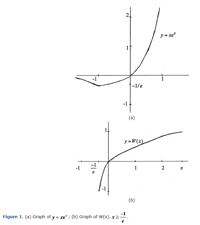
Figure 1. (a) Graph of f(x)=xexf (x) = x e^xf(x)=xex; (b) Graph of W(x)W (x)W(x), x∈[−1/e,+∞)x \in [-1/e, +\infty)x∈[−1/e,+∞).
图 1. (a) 函数 f(x)=xexf (x) = x e^xf(x)=xex 的图像;(b) 函数 W(x)W (x)W(x) 的图像(x∈[−1/e,+∞)x \in [-1/e, +\infty)x∈[−1/e,+∞))。
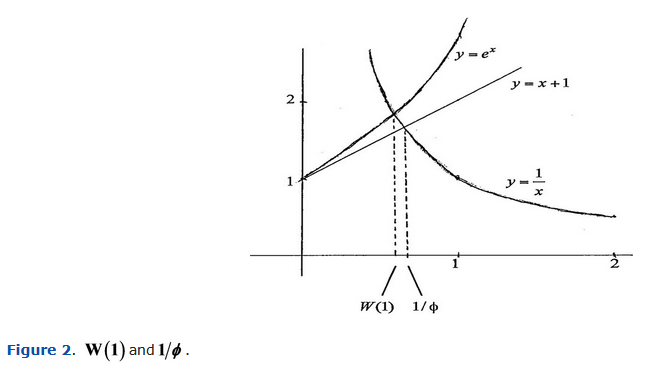
Several function values of W are easy to compute, such as W(−1e)=−1W(-\frac{1}{e}) = -1W(−e1)=−1, W(0)=0W(0) = 0W(0)=0, W(−12ln2)=−ln2W(-\frac{1}{2} \ln 2) = -\ln 2W(−21ln2)=−ln2 and W(e)=1W(e) = 1W(e)=1. The value of W(1)W(1)W(1), known as the omega constant, has the approximate value 0.567143. The number W(1)W(1)W(1) is, in some sense, a distant cousin of the golden ratio ϕ\phiϕ, since 1ϕ\frac{1}{\phi}ϕ1 is a solution to 1x=x+1\frac{1}{x} = x + 1x1=x+1, and W(1)W(1)W(1) is the solution to 1x=ex\frac{1}{x} = e^{x}x1=ex, and x+1x + 1x+1 is the linear Maclaurin approximation to exe^{x}ex (Figure 2). Since W is the inverse of xexx e^{x}xex, it follows that W(1)eW(1)=1W(1) e^{W(1)} = 1W(1)eW(1)=1 and that the slope of the curve in Figure 1(b) at the point (1,W(1))(1, W(1))(1,W(1)) is [1+eW(1)]−1≈0.6381[1 + e^{W(1)}]^{-1} ≈ 0.6381[1+eW(1)]−1≈0.6381.
W 函数的部分函数值易于计算,例如 W(−1e)=−1W(-\frac{1}{e}) = -1W(−e1)=−1、W(0)=0W(0) = 0W(0)=0、W(−12ln2)=−ln2W(-\frac{1}{2} \ln 2) = -\ln 2W(−21ln2)=−ln2 及 W(e)=1W(e) = 1W(e)=1。其中 W(1)W(1)W(1) 被称为“欧米伽常数”,近似值为 0.567143。从某种意义上看,W(1)W(1)W(1) 是黄金比例 ϕ\phiϕ 的“远亲”:因为 1ϕ\frac{1}{\phi}ϕ1 是方程 1x=x+1\frac{1}{x} = x + 1x1=x+1 的解,而 W(1)W(1)W(1) 是方程 1x=ex\frac{1}{x} = e^{x}x1=ex 的解,且 x+1x + 1x+1 恰为 exe^{x}ex 的线性麦克劳林近似(图 2)。由于 W 函数是 xexx e^{x}xex 的反函数,由此可推出 W(1)eW(1)=1W(1) e^{W(1)} = 1W(1)eW(1)=1,且图 1(b) 中曲线在点 (1,W(1))(1, W(1))(1,W(1)) 处的斜率为 [1+eW(1)]−1≈0.6381[1 + e^{W(1)}]^{-1} ≈ 0.6381[1+eW(1)]−1≈0.6381。
3. Computation
3. 计算方法
A natural question is how to compute arbitrary values of W(x)W(x)W(x). One result, from the Lagrange inversion theorem, asserts that the Lambert W function has the Taylor series expansion [6,7]
一个自然的问题是:如何计算 W(x)W(x)W(x) 的任意取值?根据拉格朗日反演定理,朗伯 W 函数具有如下泰勒级数展开式[6,7]:
W(x)=∑n=1∞(−n)n−1n!xn,(1)W(x) = \sum_{n=1}^{\infty} \frac{(-n)^{n-1}}{n!} x^{n},\tag{1}W(x)=n=1∑∞n!(−n)n−1xn,(1)
which, unfortunately, has a radius of convergence of merely 1e\frac{1}{e}e1. Since the denominator n!n!n! grows rapidly, it’s advantageous to write the series with the coefficients defined recursively as
但遗憾的是,该级数的收敛半径仅为 1e\frac{1}{e}e1。由于分母 n!n!n! 增长迅速,将级数改写为系数递归定义的形式会更有利:即
W(x)=∑n=1∞cnxnW(x) = \sum_{n=1}^{\infty} c_{n} x^{n}W(x)=n=1∑∞cnxn,
with c1=1c_{1} = 1c1=1, cn=−n−1ncn−1c_{n} = -\frac{n - 1}{n} c_{n - 1}cn=−nn−1cn−1 for all n≥2n ≥ 2n≥2.
其中 c1=1c_{1} = 1c1=1,且对所有 n≥2n ≥ 2n≥2 有 cn=−n−1ncn−1c_{n} = -\frac{n - 1}{n} c_{n - 1}cn=−nn−1cn−1。
This recursion lends itself to easy programming evaluation. Testing this, with say a series of 150 terms (which is plenty, considering that ∣x∣≤1e|x| ≤ \frac{1}{e}∣x∣≤e1), with x=−12ln2≈−0.3465736x = -\frac{1}{2} \ln 2 ≈ -0.3465736x=−21ln2≈−0.3465736, we obtain a partial sum value of S=−0.69314684S = -0.69314684S=−0.69314684, which differs from the exact value of −ln2-\ln 2−ln2 by 0.0000003. We also note that ∣x∣<1e|x| < \frac{1}{e}∣x∣<e1, so the use of the series is justified. On the other hand, a TI-graphing calculator returns “overflow error” if we try to determine W(1)W(1)W(1), primarily since the coefficients grow rapidly.
这种递归形式便于通过编程计算。例如,取 150 项级数(考虑到 ∣x∣≤1e|x| ≤ \frac{1}{e}∣x∣≤e1,150 项已足够),当 x=−12ln2≈−0.3465736x = -\frac{1}{2} \ln 2 ≈ -0.3465736x=−21ln2≈−0.3465736 时,计算得到部分和 S=−0.69314684S = -0.69314684S=−0.69314684,与精确值 −ln2-\ln 2−ln2 的差值仅为 0.0000003。同时,由于 ∣x∣<1e|x| < \frac{1}{e}∣x∣<e1,使用该级数计算是合理的。反之,若尝试用 TI 绘图计算器计算 W(1)W(1)W(1),会出现“溢出错误”,这主要是因为级数系数增长过快。
Suppose that ∣x∣>1e|x| > \frac{1}{e}∣x∣>e1 and we wish to compute W(x)W(x)W(x). One possibility is the series
若 ∣x∣>1e|x| > \frac{1}{e}∣x∣>e1 且需计算 W(x)W(x)W(x),可考虑如下级数:
W(x)=lnx−ln(lnx)+∑n=1∞(−1)n(lnx)nan(x),(2)W(x) = \ln x - \ln (\ln x) + \sum_{n=1}^{\infty} \frac{(-1)^{n}}{(\ln x)^{n}} a_{n}(x),\tag{2}W(x)=lnx−ln(lnx)+n=1∑∞(lnx)n(−1)nan(x),(2)
where 其中
an(x)=∑m=1n(−1)mS(n,n−m+1)[ln(lnx)]mm!a_{n}(x) = \sum_{m=1}^{n} (-1)^{m} S(n, n - m + 1) \frac{[\ln (\ln x)]^{m}}{m!}an(x)=m=1∑n(−1)mS(n,n−m+1)m![ln(lnx)]m
and S(n,k)S(n, k)S(n,k) denotes a Stirling number of the first kind [3].
且 S(n,k)S(n, k)S(n,k) 表示第一类斯特林数[3]。
The series (2) is somewhat impractical to use because of the difficulty in determining an(x)a_{n}(x)an(x); it turns out to be more useful to employ some standard numerical schemes for approximating W(x)W(x)W(x).
由于确定 an(x)a_{n}(x)an(x) 存在困难,该级数(2)的实用性有限;事实上,采用标准数值方法近似计算 W(x)W(x)W(x) 会更有效。
First, setting W(x)=yW(x) = yW(x)=y, we need to solve yey=xy e^{y} = xyey=x. Defining the function ggg by g(y)=yey−xg(y) = y e^{y} - xg(y)=yey−x, we use Newton’s method to approximate yyy in g(y)=0g(y) = 0g(y)=0. This gives
首先,令 W(x)=yW(x) = yW(x)=y,则需求解方程 yey=xy e^{y} = xyey=x。定义函数 g(y)=yey−xg(y) = y e^{y} - xg(y)=yey−x,采用牛顿法近似求解 g(y)=0g(y) = 0g(y)=0 的根,迭代公式为:
yn+1=yn−g(yn)g′(yn)=yn2+xe−ynyn+1.y_{n+1} = y_{n} - \frac{g(y_{n})}{g'(y_{n})} = \frac{y_{n}^{2} + x e^{-y_{n}}}{y_{n} + 1}.yn+1=yn−g′(yn)g(yn)=yn+1yn2+xe−yn..
To determine W(2)W(2)W(2), for example, starting with an initial approximate of y0=0y_{0} = 0y0=0, after 7 more iterations we get y8=0.852605502y_{8} = 0.852605502y8=0.852605502, which is an excellent approximation to W(2)W(2)W(2) because y8ey8y_{8} e^{y_{8}}y8ey8 returns 2 on the calculator. If xxx is a relatively small number, then an initial approximate of 0 will suffice for the algorithm; but if xxx is large, then lnx\ln xlnx can be chosen for y0y_{0}y0. For instance, if x=10x = 10x=10, choose y0=ln10≈2.302585y_{0} = \ln 10 ≈ 2.302585y0=ln10≈2.302585, and after 5 iterations we get W(10)≈1.745528003W(10) ≈ 1.745528003W(10)≈1.745528003.
以计算 W(2)W(2)W(2) 为例:取初始近似值 y0=0y_{0} = 0y0=0,经过 7 次迭代后得到 y8=0.852605502y_{8} = 0.852605502y8=0.852605502——该值是 W(2)W(2)W(2) 的优良近似,因为计算器计算 y8ey8y_{8} e^{y_{8}}y8ey8 的结果为 2。若 xxx 是较小的数,取初始近似值 0 即可满足算法需求;若 xxx 较大,则可选择 y0=lnxy_{0} = \ln xy0=lnx。例如,当 x=10x = 10x=10 时,取 y0=ln10≈2.302585y_{0} = \ln 10 ≈ 2.302585y0=ln10≈2.302585,经过 5 次迭代后得到 W(10)≈1.745528003W(10) ≈ 1.745528003W(10)≈1.745528003。
Newton’s method is a favorite iteration scheme for many because of its simplicity, though the convergence, quadratic in general, is typically relatively slow. A faster choice is furnished by Halley’s method (of Halley’s comet fame), which produces cubic convergence, and happens to be the choice implemented by the software Maple; this scheme gives [8]
牛顿法因原理简单成为许多人的首选迭代方法,但其收敛性通常为二次收敛,速度相对较慢。更快的选择是哈雷法(因哈雷彗星而闻名),该方法具有三次收敛性,且恰为软件 Maple 所采用的计算方案[8],其迭代公式为:
yn+1=yn−yneyn−x(yn+1)eyn−(yn+2)(yneyn−x)2yn+2.y_{n+1} = y_n - \frac{y_n e^{y_n} - x}{(y_n + 1)e^{y_n} - \frac{(y_n + 2)(y_n e^{y_n} - x)}{2y_n + 2}}. yn+1=yn−(yn+1)eyn−2yn+2(yn+2)(yneyn−x)yneyn−x.
Employing this gives W(10)≈1.745528003W(10) ≈ 1.745528003W(10)≈1.745528003 after 3 iterations. This complex looking scheme is actually what you get when you apply Newton’s method to the function g(y)g′(y)\frac{g(y)}{\sqrt{g'(y)}}g′(y)g(y) [9]. An alternative root-finding scheme, using continued fraction expansion, is described in [10].
采用该方法计算 W(10)W(10)W(10) 时,仅需 3 次迭代即可得到 W(10)≈1.745528003W(10) ≈ 1.745528003W(10)≈1.745528003。这一看似复杂的方案,本质上是对函数 g(y)g′(y)\frac{g(y)}{\sqrt{g'(y)}}g′(y)g(y) 应用牛顿法的结果[9]。文献[10] 还介绍了另一种基于连分数展开的求根方法。
4. Calculus
4. 微积分性质
We know that since y=xexy = x e^{x}y=xex is an increasing and differentiable function for all x>−1x > -1x>−1, then its inverse y=W(x)y = W(x)y=W(x) is likewise increasing and differentiable for all x>−1ex > -\frac{1}{e}x>−e1. Differentiating x=yeyx = y e^{y}x=yey with respect to yyy, we obtain
已知函数 y=xexy = x e^{x}y=xex 在所有 x>−1x > -1x>−1 的范围内是单调递增且可微的,因此其反函数 y=W(x)y = W(x)y=W(x) 在所有 x>−1ex > -\frac{1}{e}x>−e1 的范围内也同样单调递增且可微。对 x=yeyx = y e^{y}x=yey 关于 yyy 求导,可得
1=dWdxdxdy=dWdx[yey+ey],1 = \frac{dW}{dx} \frac{dx}{dy} = \frac{dW}{dx} \left[ y e^y + e^y \right], 1=dxdWdydx=dxdW[yey+ey],
so
因此
W′(x)=1(y+1)ey=y(y+1)yey=y(y+1)x=W(x)[W(x)+1]x=e−W(x)1+W(x),x≠0.(3)\begin{aligned} W'(x) &= \frac{1}{(y+1)e^y} = \frac{y}{(y+1)ye^y}\\ &= \frac{y}{(y+1)x} = \frac{W(x)}{[W(x) + 1]x} = \frac{e^{-W(x)}}{1 + W(x)}, \quad x \neq 0. \end{aligned} \tag{3}W′(x)=(y+1)ey1=(y+1)yeyy=(y+1)xy=[W(x)+1]xW(x)=1+W(x)e−W(x),x=0.(3)
In particular,
特别地
W′(e)=1e(1+1)=12eW'(e) = \frac{1}{e(1 + 1)} = \frac{1}{2e}W′(e)=e(1+1)1=2e1,
and similarly,
同理,
limx→(−1e)+W′(x)=∞\lim_{x \to (-\frac{1}{e})^+} W'(x) = \inftylimx→(−e1)+W′(x)=∞.
What about W′(0)W'(0)W′(0)? The right-hand side of (3)(3)(3) is indeterminant at x=0x = 0x=0, but division of both sides of (1)(1)(1) by xxx and taking the limit as x→0x \to 0x→0 give
那么 W′(0)W'(0)W′(0) 如何计算?(3)(3)(3) 在 x=0x = 0x=0 处为不定式,但将 (1)(1)(1) 两边同除以 xxx 并取 x→0x \to 0x→0 的极限,可得
limx→0W(x)eW(x)x=1.\lim_{x \to 0} \frac{W(x) e^{W(x)}}{x} = 1. x→0limxW(x)eW(x)=1.
Since limx→0eW(x)=e0=1\lim_{x \to 0} e^{W(x)} = e^{0} = 1limx→0eW(x)=e0=1, this yields limx→0W(x)x=1\lim_{x \to 0} \frac{W(x)}{x} = 1limx→0xW(x)=1. Thus,
由于 limx→0eW(x)=e0=1\lim_{x \to 0} e^{W(x)} = e^{0} = 1limx→0eW(x)=e0=1,因此 limx→0W(x)x=1\lim_{x \to 0} \frac{W(x)}{x} = 1limx→0xW(x)=1,进而有:
W′(0)=limx→0W(x)x[1+W(x)]=limx→0W(x)/x1+W(x)=11=1.W'(0) = \lim_{x \to 0} \frac{W(x)}{x \left[ 1 + W(x) \right]} = \lim_{x \to 0} \frac{W(x)/x}{1 + W(x)} = \frac{1}{1}= 1. W′(0)=x→0limx[1+W(x)]W(x)=x→0lim1+W(x)W(x)/x=11=1.
For large xxx, the graph of W(x)W(x)W(x) bears strong resemblance to lnx\ln xlnx, since from (2) we have limx→∞W(x)lnx=1\lim_{x \to \infty} \frac{W(x)}{\ln x} = 1limx→∞lnxW(x)=1 although we have to be careful here because the difference ∣W(x)−lnx∣|W(x) - \ln x|∣W(x)−lnx∣ increases without bound as x→∞x \to \inftyx→∞ [7]. The graph of W(x)W(x)W(x), like that of lnx\ln xlnx, is concave downward for all xxx since xexxe^xxex is concave upward. If we differentiate (3), and omit the argument xxx for brevity, then
对于较大的 xxx,W(x)W(x)W(x) 的图像与 lnx\ln xlnx 非常相似,因为从公式 (2) 我们有 limx→∞W(x)lnx=1\lim_{x \to \infty} \frac{W(x)}{\ln x} = 1limx→∞lnxW(x)=1,尽管我们必须小心,因为差值 ∣W(x)−lnx∣|W(x) - \ln x|∣W(x)−lnx∣ 随着 x→∞x \to \inftyx→∞ 无限增加 [7]。W(x)W(x)W(x) 的图像,像 lnx\ln xlnx 一样,对于所有的 xxx 都是向下凹的,因为 xexxe^xxex 是向上凹的。如果我们对公式 (3) 求导,并为了简洁省略参数 xxx,那么
W′′=x(1+W)W′−W[xW′+1+W]x2(1+W)2=−2W2−W3x2(1+W)3<0.W'' = \frac{x(1+W)W' - W[xW' + 1 + W]}{x^2(1+W)^2} = \frac{-2W^2 - W^3}{x^2(1+W)^3} < 0. W′′=x2(1+W)2x(1+W)W′−W[xW′+1+W]=x2(1+W)3−2W2−W3<0.
Rewriting W′′W''W′′ as e−2W[−(W+2)](1+W)3\frac{e^{-2W}\left[-(W+2)\right]}{(1+W)^3}(1+W)3e−2W[−(W+2)] puts this into the form which fits the general case for W(n)W^{(n)}W(n) [5]. In fact, from this form, we readily see that there is a point of inflection on the curve when W=−2W = -2W=−2, which actually falls on the other branch of the WWW function.
将 W′′W''W′′ 重写为 e−2W[−(W+2)](1+W)3\frac{e^{-2W}\left[-(W+2)\right]}{(1+W)^3}(1+W)3e−2W[−(W+2)] 使其符合 W(n)W^{(n)}W(n) 的一般情况 [5]。实际上,从这种形式,我们很容易看出当 W=−2W = -2W=−2 时,曲线上有一个拐点,这实际上落在 WWW 函数的另一个分支上。
Continuing along the calculus vein, we should examine, if possible, the integral of W(x)W(x)W(x). To this end, recall that y=W(x)y = W(x)y=W(x) iff x=yeyx = y e^{y}x=yey. Thus, dx=ey(1+y)dydx = e^{y}(1 + y) dydx=ey(1+y)dy, and
接下来从微积分角度进一步分析,若可能,还需研究 W(x)W(x)W(x) 的积分。为此,回顾 y=W(x)y = W(x)y=W(x) 当且仅当 x=yeyx = y e^{y}x=yey,因此 dx=ey(1+y)dydx = e^{y}(1 + y) dydx=ey(1+y)dy,进而有:
∫W(x)dx=∫ydyW′(x)=∫ydyW(x)x(1+W(x))=∫[yey+y2ey]dy\begin{aligned} \int W(x) \, dx &= \int y \frac{dy}{W'(x)} = \int \frac{y \, dy}{W(x)} x(1 + W(x))\\ &= \int \left[ ye^y + y^2 e^y \right] \, dy \end{aligned}∫W(x)dx=∫yW′(x)dy=∫W(x)ydyx(1+W(x))=∫[yey+y2ey]dy
and integrating this last integral by parts, we obtain
并使用分部积分法计算最后一个积分,我们得到
x[y−1+1y],x \left[ y - 1 + \frac{1}{y} \right], x[y−1+y1],
which now gives
这现在给出了
∫W(x)dx=x[W(x)−1+1W(x)]+C.(4)\int W(x) \, dx = x \left[ W(x) - 1 + \frac{1}{W(x)} \right] + C. \tag{4} ∫W(x)dx=x[W(x)−1+W(x)1]+C.(4)
In particular, the area of the region bounded by the curve W(x)W(x)W(x), the x-axis, and the line x=εx = \varepsilonx=ε is, therefore,
特别地,由曲线 W(x)W(x)W(x),x轴和直线 x=εx = \varepsilonx=ε 围成的区域的面积因此为,
∫0εW(x)dx=x[W(x)−1+1W(x)]∣0ε=ε[1−1+1]−limε→0ε[W(ε)−1+1W(ε)]=e−1.\begin{aligned} \int_{0}^{\varepsilon} W(x) \, dx &= x \left[ W(x) - 1 + \frac{1}{W(x)} \right] \bigg|_{0}^{\varepsilon}\\&= \varepsilon \left[ 1 - 1 + 1 \right] - \lim_{\varepsilon \to 0} \varepsilon \left[ W(\varepsilon) - 1 + \frac{1}{W(\varepsilon)} \right]\\& = e - 1.\end{aligned}∫0εW(x)dx=x[W(x)−1+W(x)1]0ε=ε[1−1+1]−ε→0limε[W(ε)−1+W(ε)1]=e−1.
We note this result agrees with evaluating the integral via inverse functions [11], because then
我们注意到这个结果与通过反函数[11]计算积分是一致的,因为
∫0eW(x)dx=eW(e)−0W(0)−∫0W(e)xexdx=e−1.\int_{0}^{e} W(x) \, dx = e \, W(e) - 0 \, W(0) - \int_{0}^{W(e)} x e^x \, dx = e - 1. ∫0eW(x)dx=eW(e)−0W(0)−∫0W(e)xexdx=e−1.
Other integrals, involving functions containing WWW, can be computed, some just with a special change of variable [6]. For instance,
涉及 WWW 的其他积分可以计算,有些只需通过变量的特殊变换[6]。例如,
∫xW(x)dx=12e2W(x)[W(x)−12[W2(x)+12]+C].\int x W(x) \, dx = \frac{1}{2} e^{2W(x)} \left[ W(x) - \frac{1}{2} \left[ W^2(x) + \frac{1}{2} \right] + C \right]. ∫xW(x)dx=21e2W(x)[W(x)−21[W2(x)+21]+C].
The function xW(x)xW(x)xW(x) is concave up, connecting (0,0)(0,0)(0,0)
函数 xW(x)xW(x)xW(x) 是向上凹的,连接 (0,0)(0,0)(0,0)
and (e,e)(e, e)(e,e), hence its area KaTeX parse error: Expected 'EOF', got '\right' at position 55: …{(3e^2 + 1)/8} \̲r̲i̲g̲h̲t̲) is less than ∫0exdx=e22\int_{0}^{e} x \, dx = \frac{e^2}{2}∫0exdx=2e2. Similarly we find
和 (e,e)(e, e)(e,e),因此其面积 KaTeX parse error: Expected 'EOF', got '\right' at position 55: …{(3e^2 + 1)/8} \̲r̲i̲g̲h̲t̲) 小于 ∫0exdx=e22\int_{0}^{e} x \, dx = \frac{e^2}{2}∫0exdx=2e2。同样我们发现
∫0exW(x)dx=14e2W(x)[1+2W(x)]∣0e=3e24,\int_{0}^{e} \frac{x}{W(x)} \, dx = \frac{1}{4} e^{2W(x)} \left[ 1 + 2W(x) \right] \bigg|_{0}^{e} = \frac{3e^2}{4}, ∫0eW(x)xdx=41e2W(x)[1+2W(x)]0e=43e2,
and this is greater than e22\frac{e^2}{2}2e2 since x/W(x)x/W(x)x/W(x) is increasing and concave down from (0,1)(0,1)(0,1) to (e,e)(e, e)(e,e).
这大于 e22\frac{e^2}{2}2e2,因为 x/W(x)x/W(x)x/W(x) 从 (0,1)(0,1)(0,1) 到 (e,e)(e, e)(e,e) 是递增且向下凹的。
5. Applications
5. 应用领域
An article appeared in the February, 2000, issue of FOCUS, the newsletter of the Mathematical Association of America, touting the merits of the W function as a candidate for a new elementary function to be studied in schools and to be included in textbooks [12]. The rationale for this was that not only is W a radically different function from the traditional elementary functions of polynomials, rationals, exponentials, logarithmics, and trigonometrics, but its calculus provides a wealth of interesting, and powerful, applications. A number of these are mentioned in a paper by Corless et al., where they describe such applications as enumeration of trees, combustion, enzyme kinetics, linear delay equations, population growth, spread of disease, and the analysis of algorithms [3]. An article [13] by Packel and Yuen shows that W is instrumental in determining the maximum range for a projectile with linear resistance (problems of this type have certainly been important for several thousand years). The solution for the current in a series diode/resistor circuit can also be written in terms of W. Applications of W are found in complex cases involving atomic, nuclear, and optical physics. The first physics problem to be solved explicitly in terms of W was one in which the exchange forces between two nuclei within the hydrogen molecular ion (H2+)(H_2^+)(H2+) were calculated [14].
2000 年 2 月,美国数学协会通讯《聚焦》(FOCUS)刊登了一篇文章,宣扬朗伯 W 函数作为“新基本函数”的优势,认为其应纳入学校教学内容并收录进教材[12]。理由如下:W 函数不仅与多项式、有理函数、指数函数、对数函数、三角函数等传统基本函数截然不同,其微积分性质还衍生出丰富有趣且实用性强的应用。科莱斯等人的论文中提及了多个应用场景,包括树的计数、燃烧学、酶动力学、线性时滞方程、种群增长、疾病传播及算法分析[3]。帕克尔与袁合著的文章[13] 指出,W 函数对确定“线性阻力下抛射体的最大射程”起关键作用(这类问题数千年来一直具有重要意义);此外,二极管/电阻串联电路的电流解也可通过 W 函数表示。在复杂场景中,W 函数的应用还涉及原子物理、核物理与光学:首个明确用 W 函数求解的物理问题,是计算氢分子离子 (H2+)(H_2^+)(H2+) 内两个原子核之间的交换力[14]。
Several other cases involve generalized Gaussian noise, solar winds, black holes, general relativity, quantum chromodynamics, fuel consumption, Stirling’s formula for n!n!n!, cardiorespiratory control, water-wave heights in oceanography, enumeration of trees in combinatorics, and statistical mechanics [5,15-17]. A really interesting analog of W(x)W(x)W(x) is given by Dan Kalman [18], where he defines a function glog, similar to W, in that glog is the inverse to exx\frac{e^{x}}{x}xex. The glog function bears a strong resemblance to W(x)W(x)W(x), possessing similar properties and useful common applications, such as solving exponential-linear equations. The two functions are intimately related by W(x)=−glog(−1x)and glog(x)=−W(−1x)W(x) = -g\mathrm{log}(-\frac{1}{x})\ \text{and} \ g\mathrm{log}(x) = -W(-\frac{1}{x})W(x)=−glog(−x1) and glog(x)=−W(−x1).
其他应用场景还包括:广义高斯噪声、太阳风、黑洞、广义相对论、量子色动力学、燃料消耗、n!n!n! 的斯特林公式、心肺调节、海洋学中的水波高度、组合数学中的树计数及统计力学[5,15-17]。丹·卡尔曼[18] 提出了一个与 W(x)W(x)W(x) 十分相似的函数——glog 函数:glog 是 exx\frac{e^{x}}{x}xex 的反函数,与 W(x)W(x)W(x) 性质相似且存在共同实用场景(如求解指数-线性方程)。两者通过以下关系式紧密关联: W(x)=−glog(−1x)及 glog(x)=−W(−1x)。W(x) = -g\mathrm{log}(-\frac{1}{x}) \ 及 \ g\mathrm{log}(x) = -W(-\frac{1}{x})。W(x)=−glog(−x1) 及 glog(x)=−W(−x1)。
6. Algebra
6. 代数应用
In a high-school precalculus course one might be presented with the elementary equation 2x=102^x = 102x=10 to solve. Now, instead, let’s solve a similar equation 2x=10x2^x = 10x2x=10x, which means that it won’t suffice to begin by taking the logarithm of both sides. Instead, we proceed as follows:
高中预备微积分课程中可能会涉及求解基本方程 2x=102^x = 102x=10。现在我们来求解一个类似方程 2x=10x2^x = 10x2x=10x——该方程无法通过“对两边取对数”直接求解,需按以下步骤进行:
2x=10x↔1=10x⋅2−x=10xe−xln2↔−ln210=−xln2⋅e−xln22^x = 10x \leftrightarrow 1 = 10x \cdot 2^{-x} = 10x e^{-x \ln 2} \leftrightarrow -\frac{\ln 2}{10} = -x \ln 2 \cdot e^{-x \ln 2}2x=10x↔1=10x⋅2−x=10xe−xln2↔−10ln2=−xln2⋅e−xln2
Since the right-hand side of this last equation is of the form zezz e^zzez, and since we know z=W(y)z = W(y)z=W(y) if y=zezy = z e^zy=zez, then −xln2=W(−ln210)-x \ln 2 = W(-\frac{\ln 2}{10})−xln2=W(−10ln2), or
上式右边为 zezz e^zzez 形式,而由 y=zezy = z e^zy=zez 可知 z=W(y)z = W(y)z=W(y),因此 −xln2=W(−ln210)-x \ln 2 = W(-\frac{\ln 2}{10})−xln2=W(−10ln2),即
x=−W(−ln210)ln2x = -\frac{W(-\frac{\ln 2}{10})}{\ln 2}x=−ln2W(−10ln2).
Using the Taylor series (1) to approximate W(−110ln2)W(-\frac{1}{10} \ln 2)W(−101ln2) (since ∣−110ln2∣≈0.069<1e|-\frac{1}{10} \ln 2| ≈ 0.069 < \frac{1}{e}∣−101ln2∣≈0.069<e1), we get
由于 ∣−110ln2∣≈0.069<1e|-\frac{1}{10} \ln 2| ≈ 0.069 < \frac{1}{e}∣−101ln2∣≈0.069<e1,可使用泰勒级数(1)近似计算 W(−110ln2)W(-\frac{1}{10} \ln 2)W(−101ln2),得到
W(−110ln2)≈−0.0746900848W(-\frac{1}{10} \ln 2) ≈ -0.0746900848W(−101ln2)≈−0.0746900848,
so
因此
x≈0.0746900848ln2≈0.1077550149x ≈ \frac{0.0746900848}{\ln 2} ≈ 0.1077550149x≈ln20.0746900848≈0.1077550149.
Checking, we find
验证可知
2x≈20.1077550149≈1.07755015=10x2^x ≈ 2^{0.1077550149} ≈ 1.07755015 = 10x2x≈20.1077550149≈1.07755015=10x,
which confirms the solution.
该解成立。
The equation 2x=10x2^x = 10x2x=10x is a special case of a more general setting abx+c=dx+ea^{bx + c} = dx + eabx+c=dx+e, where we assume the base a>0a > 0a>0 and where neither bbb nor ddd equals zero. The substitution t=bx+et = bx + et=bx+e gives
方程 2x=10x2^x = 10x2x=10x 是更一般方程 abx+c=dx+ea^{bx + c} = dx + eabx+c=dx+e 的特殊情况,其中底数 a>0a > 0a>0,且 bbb、ddd 均不为零。令 t=bx+et = bx + et=bx+e,则:
abx+c=a−t+e+c=d(t−eb)+e=dtb−deb+ea^{bx + c} = a^{-t + e + c} = d\left(\frac{t - e}{b}\right) + e = \frac{d t}{b} - \frac{d e}{b} + eabx+c=a−t+e+c=d(bt−e)+e=bdt−bde+e
and, thus, multiplying both sides by lna\ln alna gives
两边同乘 lna\ln alna,可得:
−bd(lna)ac−bed=t(lna)etlna-\frac{b}{d} (\ln a) a^{c - \frac{b e}{d}} = t (\ln a) e^{t \ln a}−db(lna)ac−dbe=t(lna)etlna
which now has the form u=wewu = w e^wu=wew, so w=W(u)w = W(u)w=W(u) or tlna=W(−bdlna⋅ac−bed)t \ln a = W\left(-\frac{b}{d} \ln a \cdot a^{c - \frac{b e}{d}}\right)tlna=W(−dblna⋅ac−dbe), and hence
上式右边为 u=wewu = w e^wu=wew 形式,因此 w=W(u)w = W(u)w=W(u),即 tlna=W(−bdlna⋅ac−bed)t \ln a = W\left(-\frac{b}{d} \ln a \cdot a^{c - \frac{b e}{d}}\right)tlna=W(−dblna⋅ac−dbe),进而有:
x=t−eb=1blnaW(−bdlna⋅ac−bed)−ebx = \frac{t - e}{b} = \frac{1}{b \ln a} W\left(-\frac{b}{d} \ln a \cdot a^{c - \frac{b e}{d}}\right) - \frac{e}{b}x=bt−e=blna1W(−dblna⋅ac−dbe)−be.
Another interesting algebraic application involves the infinite tower of exponents xxx⋅⋅x^{x^{x^{\cdot^{\cdot}}}}xxx⋅⋅, which will be denoted by T(x)T(x)T(x). To solve the particular equation T(x)=2T(x) = 2T(x)=2, one might argue that this is equivalent to xT(x)=2x^{T(x)} = 2xT(x)=2, in which case x2=2x^2 = 2x2=2, so x=2x = \sqrt{2}x=2, which is the correct solution to T(x)=2T(x) = 2T(x)=2. But what about T(x)=4T(x) = 4T(x)=4? It stands to reason that as yyy increases, so does xxx in T(x)=yT(x) = yT(x)=y. But with T(x)=4T(x) = 4T(x)=4, we can write this as xT(x)=4x^{T(x)} = 4xT(x)=4, or x4=4x^4 = 4x4=4, so x=2x = \sqrt{2}x=2 again! Something isn’t right.
另一有趣的代数应用涉及无穷指数塔 xxx⋅⋅x^{x^{x^{\cdot^{\cdot}}}}xxx⋅⋅,记为 T(x)T(x)T(x)。求解方程 T(x)=2T(x) = 2T(x)=2 时,可认为其等价于 xT(x)=2x^{T(x)} = 2xT(x)=2,即 x2=2x^2 = 2x2=2,因此 x=2x = \sqrt{2}x=2——这是 T(x)=2T(x) = 2T(x)=2 的正确解。但求解 T(x)=4T(x) = 4T(x)=4 时会出现矛盾:按常理,在 T(x)=yT(x) = yT(x)=y 中,yyy 增大时 xxx 也应增大;但由 T(x)=4T(x) = 4T(x)=4 可得 xT(x)=4x^{T(x)} = 4xT(x)=4,即 x4=4x^4 = 4x4=4,再次得到 x=2x = \sqrt{2}x=2,显然存在问题。
The underlying problem is with the domain of TTT. We find in [19] that the infinite tower of exponents is only defined (i.e., finite) on its interval of convergence 1ee≤x≤e1e\frac{1}{e^e} ≤ x ≤ e^{\frac{1}{e}}ee1≤x≤ee1, or approximately 0.065988<x<1.4446670.065988 < x < 1.4446670.065988<x<1.444667. So if xxx is selected from this interval, what is T(x)T(x)T(x)? If we set T(x)=yT(x) = yT(x)=y, then
问题根源在于 T(x)T(x)T(x) 的定义域。文献[19] 指出,无穷指数塔仅在收敛区间 1ee≤x≤e1e\frac{1}{e^e} ≤ x ≤ e^{\frac{1}{e}}ee1≤x≤ee1(近似为 0.065988<x<1.4446670.065988 < x < 1.4446670.065988<x<1.444667)内有定义(即取值有限)。若 xxx 属于该区间,T(x)T(x)T(x) 的值如何确定?令 T(x)=yT(x) = yT(x)=y,则:
xT(x)=y↔lnx⋅eylnx=ylnx↔W(−lnx)=−ylnx↔y=W(−lnx)−lnxx^{T(x)} = y \leftrightarrow \ln x \cdot e^{y \ln x} = y \ln x \leftrightarrow W(-\ln x) = -y \ln x \leftrightarrow y = \frac{W(-\ln x)}{-\ln x}xT(x)=y↔lnx⋅eylnx=ylnx↔W(−lnx)=−ylnx↔y=−lnxW(−lnx)
Note also that y=1y = 1y=1 when x=1x = 1x=1, and the above expression for yyy gives a function continuous at x=1x = 1x=1, since limu→0W(u)u=1\lim_{u \to 0} \frac{W(u)}{u} = 1limu→0uW(u)=1.
需注意,当 x=1x = 1x=1 时 y=1y = 1y=1,且上述表达式在 x=1x = 1x=1 处连续——因为 limu→0W(u)u=1\lim_{u \to 0} \frac{W(u)}{u} = 1limu→0uW(u)=1。
Hence if 1ee≤x≤e1e\frac{1}{e^e} ≤ x ≤ e^{\frac{1}{e}}ee1≤x≤ee1, then e≥−lnx≥−1ee ≥ -\ln x ≥ -\frac{1}{e}e≥−lnx≥−e1, so 1e≤y≤e\frac{1}{e} ≤ y ≤ ee1≤y≤e, and this is why the equation T(x)=2T(x) = 2T(x)=2 is solvable (since 2≤e2 ≤ e2≤e), but T(x)=4T(x) = 4T(x)=4 is not (since 4>e4 > e4>e).
因此,若 1ee≤x≤e1e\frac{1}{e^e} ≤ x ≤ e^{\frac{1}{e}}ee1≤x≤ee1,则 e≥−lnx≥−1ee ≥ -\ln x ≥ -\frac{1}{e}e≥−lnx≥−e1,进而 1e≤y≤e\frac{1}{e} ≤ y ≤ ee1≤y≤e。这就是为何 T(x)=2T(x) = 2T(x)=2 可解(因 2≤e2 ≤ e2≤e),而 T(x)=4T(x) = 4T(x)=4 无解(因 4>e4 > e4>e)。
The graph of TTT is an increasing function with domain [1ee,e1e][\frac{1}{e^e}, e^{\frac{1}{e}}][ee1,ee1] and range [1e,e][\frac{1}{e}, e][e1,e]. It also passes through the two obvious points (1,1)(1, 1)(1,1) and (1e,W(1))≈(1e,0.567143)(\frac{1}{e}, W(1)) ≈ (\frac{1}{e}, 0.567143)(e1,W(1))≈(e1,0.567143). What else can we deduce? Checking for differentiability, we have from the chain rule: if y=T(x)=xyy = T(x) = x^yy=T(x)=xy, then taking the natural logarithm of both sides gives lny=ylnx\ln y = y \ln xlny=ylnx. Differentiating both sides with respect to xxx gives
T(x)T(x)T(x) 的图像为单调递增函数,定义域为 [1ee,e1e][\frac{1}{e^e}, e^{\frac{1}{e}}][ee1,ee1],值域为 [1e,e][\frac{1}{e}, e][e1,e],且经过两个明显的点:(1,1)(1, 1)(1,1) 和 (1e,W(1))≈(1e,0.567143)(\frac{1}{e}, W(1)) ≈ (\frac{1}{e}, 0.567143)(e1,W(1))≈(e1,0.567143)。进一步分析可微性:由链式法则,若 y=T(x)=xyy = T(x) = x^yy=T(x)=xy,对两边取自然对数得 lny=ylnx\ln y = y \ln xlny=ylnx;对 xxx 求导得
1yy′=yx+y′lnx\frac{1}{y} y' = \frac{y}{x} + y' \ln xy1y′=xy+y′lnx, or y′=y2x−xylnxy' = \frac{y^2}{x - x y \ln x}y′=x−xylnxy2;
so again,
进而
y′=y2x(1−ylnx)y' = \frac{y^2}{x(1 - y \ln x)}y′=x(1−ylnx)y2.
Using this form for y′y'y′ to compute T′(1)T'(1)T′(1), we get T′(1)=121(1−1⋅0)=1T'(1) = \frac{1^2}{1(1 - 1 \cdot 0)} = 1T′(1)=1(1−1⋅0)12=1, and since the limit of this expression is 1 as x→1x \to 1x→1, then T′(1)=1T'(1) = 1T′(1)=1, and hence T′T'T′ is never 0, so TTT is always strictly increasing. The following small table (Table 1) of values will prove helpful.
计算 T′(1)T'(1)T′(1) 得 T′(1)=121(1−1⋅0)=1T'(1) = \frac{1^2}{1(1 - 1 \cdot 0)} = 1T′(1)=1(1−1⋅0)12=1;且当 x→1x \to 1x→1 时,该表达式的极限为 1,因此 T′(1)=1T'(1) = 1T′(1)=1。由于 T′(x)T'(x)T′(x) 恒不为 0,故 T(x)T(x)T(x) 始终严格单调递增。表 1 列出了部分导数数值,可供参考。
Table 1. Some derivative values of T(x)T(x)T(x)
表 1. T(x)T(x)T(x) 的部分导数数值
| xxx | T′(x)T'(x)T′(x) |
|---|---|
| e1ee^{\frac{1}{e}}ee1 | ∞\infty∞ |
| 111 | 111 |
| 1e\frac{1}{e}e1 | ≈0.558≈ 0.558≈0.558 |
| 1ee\frac{1}{e^e}ee1 | ≈1.025≈ 1.025≈1.025 |
| 0.3940.3940.394 | 0.5570.5570.557 |
Alternatively, we could have found T′T'T′ by implicit differentiation of y=T(x)=xyy = T(x) = x^yy=T(x)=xy. Thus 1yy′=yx+y′lnx\frac{1}{y} y' = \frac{y}{x} + y' \ln xy1y′=xy+y′lnx, or y′=y2x−xylnxy' = \frac{y^2}{x - x y \ln x}y′=x−xylnxy2; so again, y′=y2x(1−ylnx)y' = \frac{y^2}{x(1 - y \ln x)}y′=x(1−ylnx)y2. Using this form for y′y'y′ to compute y′′y''y′′ (after some algebraic manipulations and cancellations) gives,
此外,也可通过对 y=T(x)=xyy = T(x) = x^yy=T(x)=xy 隐函数求导得到 T′(x)T'(x)T′(x),结果同上:y′=y2x(1−ylnx)y' = \frac{y^2}{x(1 - y \ln x)}y′=x(1−ylnx)y2。利用该导数表达式进一步计算二阶导数 y′′y''y′′(经代数运算与消元后):
y′′=y3(2−ylnx)+y2(y−1+ylnx)(1−ylnx)x2(1−ylnx)3y'' = \frac{y^3(2 - y \ln x) + y^2(y - 1 + y \ln x)(1 - y \ln x)}{x^2(1 - y \ln x)^3}y′′=x2(1−ylnx)3y3(2−ylnx)+y2(y−1+ylnx)(1−ylnx)
This complex expression appears to yield negative values for all x<0.394x < 0.394x<0.394 and positive values for all x>0.394x > 0.394x>0.394, and
该复杂表达式在 x<0.394x < 0.394x<0.394 时取值为负,在 x>0.394x > 0.394x>0.394 时取值为正;且
y′(0.394)=0.581720.394×[1−0.5817×ln0.394]≈0.33840.394×(1+0.5817×0.9314)≈0.557y'(0.394) = \frac{0.5817^2}{0.394 \times [1 - 0.5817 \times \ln 0.394]} ≈ \frac{0.3384}{0.394 \times (1 + 0.5817 \times 0.9314)} ≈ 0.557y′(0.394)=0.394×[1−0.5817×ln0.394]0.58172≈0.394×(1+0.5817×0.9314)0.3384≈0.557.
Hence, we have an inflection point at x≈0.394x ≈ 0.394x≈0.394 (where y≈0.5817y ≈ 0.5817y≈0.5817). Putting all of these pieces of the puzzle together, we obtain a decent graph of TTT, as shown in Figure 3.
因此,曲线在 x≈0.394x ≈ 0.394x≈0.394(对应 y≈0.5817y ≈ 0.5817y≈0.5817)处存在拐点。整合上述所有信息,可得到 T(x)T(x)T(x) 的完整图像,如图 3 所示。

The tower function TTT must necessarily possess an inverse T−1T^{-1}T−1. We note that if y=T(x)y = T(x)y=T(x), then y=W(−lnx)−lnxy = \frac{W(-\ln x)}{-\ln x}y=−lnxW(−lnx), so −ylnx=W(−lnx)-y \ln x = W(-\ln x)−ylnx=W(−lnx), and hence −lnx⋅e−lnx=−lnx-\ln x \cdot e^{-\ln x} = -\ln x−lnx⋅e−lnx=−lnx (since W(z)eW(z)=zW(z) e^{W(z)} = zW(z)eW(z)=z), or −lnx=ye−y-\ln x = y e^{-y}−lnx=ye−y, so lnx=−ye−y\ln x = -y e^{-y}lnx=−ye−y, and consequently,
指数塔函数 TTT 必然存在反函数 T−1T^{-1}T−1。我们注意到,若 y=T(x)y = T(x)y=T(x),则 y=W(−lnx)−lnxy = \frac{W(-\ln x)}{-\ln x}y=−lnxW(−lnx),由此可得 −ylnx=W(−lnx)-y \ln x = W(-\ln x)−ylnx=W(−lnx);根据 W(z)eW(z)=zW(z) e^{W(z)} = zW(z)eW(z)=z 的性质,进一步有 −lnx⋅e−lnx=−lnx-\ln x \cdot e^{-\ln x} = -\ln x−lnx⋅e−lnx=−lnx,即 −lnx=ye−y-\ln x = y e^{-y}−lnx=ye−y,因此 lnx=−ye−y\ln x = -y e^{-y}lnx=−ye−y,进而推出
x=e−ye−y=(ee−y)−y=(e−e−y)yx = e^{-y e^{-y}} = (e^{e^{-y}})^{-y} = (e^{-e^{-y}})^yx=e−ye−y=(ee−y)−y=(e−e−y)y.
Wait, more simply, if y=T(x)=xyy = T(x) = x^yy=T(x)=xy, then taking both sides to the power of 1y\frac{1}{y}y1 gives x=y1yx = y^{\frac{1}{y}}x=yy1, so this inverse is T−1(y)=y1yT^{-1}(y) = y^{\frac{1}{y}}T−1(y)=yy1. Composition of the two functions gives the interesting pair of identities:
更简单地说,若 y=T(x)=xyy = T(x) = x^yy=T(x)=xy,对等式两边取 1y\frac{1}{y}y1 次幂,可得 x=y1yx = y^{\frac{1}{y}}x=yy1,因此该反函数为 T−1(y)=y1yT^{-1}(y) = y^{\frac{1}{y}}T−1(y)=yy1。两个函数的复合运算可得到以下一组有趣的恒等式:
(x1x)(x1x)⋅⋅=x,1e≤x≤e\left(x^{\frac{1}{x}}\right)^{\left(x^{\frac{1}{x}}\right)^{\cdot^{\cdot}}} = x, \quad \frac{1}{e} ≤ x ≤ e (xx1)(xx1)⋅⋅=x,e1≤x≤e
and
以及
xx⋅⋅=xx,1ee≤x≤e1ex^{x^{\cdot^{\cdot}}} = \sqrt[x]{x}, \quad \frac{1}{e^e} ≤ x ≤ e^{\frac{1}{e}} xx⋅⋅=xx,ee1≤x≤ee1
REFERENCES
参考文献
[1] J. J. Gray and L. Tilling, “Johann Heinrich Lambert, Mathematician and Scientist,” Historia Mathematica, Vol. 5, No. 1, 1978, pp. 13-41. doi:10.1016/0315-0860(78)90133-7
[1] J. J.格雷、L.蒂林,《约翰·海因里希·朗伯:数学家与科学家》,《数学史》,第 5 卷第 1 期,1978 年,第 13-41 页。doi:10.1016/0315-0860(78)90133-7
[2] B. Hays, “Why W?,” American Scientist, Vol. 93, No. 2, 2005, pp. 104-108.
[2] B.海斯,《为何是 W?》,《美国科学家》,第 93 卷第 2 期,2005 年,第 104-108 页。
[3] R. M. Corless, G. H. Gonnet, D. E. Hare, D. J. Jeffrey and D. E. Knuth, “On the Lambert W Function,” Advances in Computational Mathematics, Vol. 5, No. 1, 1996, pp. 329-359.
[3] R. M.科莱斯、G. H.冈内特、D. E.黑尔、D. J.杰弗里、D. E.克努特,《论朗伯 W 函数》,《计算数学进展》,第 5 卷第 1 期,1996 年,第 329-359 页。
[4] L. Euler, “De Formulis Exponentialibus Replicatis,” Leonhardi Euleri Opera Omnia, Ser. 1, Opera Mathematica, Vol. 15, 1927, pp. 268-297.
[4] L.欧拉,《论重复指数形式》,《欧拉全集》,第 1 辑(数学著作),第 15 卷,1927 年,第 268-297 页。
[5] F. Chaspeau-Blondeau and A. Monir, “Numerical Evaluation of the Lambert W Function and Application to Generation of Generalized Gaussian Noise with Exponent ½,” IEEE Transactions on Signal Processing, Vol. 50, No. 10, 2002, pp. 2160-2165. doi:10.1109/TSP.2002.801912
[5] F.沙斯波-布朗多、A.莫尼尔,《朗伯 W 函数的数值计算及其在生成指数为 1/2 的广义高斯噪声中的应用》,《IEEE 信号处理汇刊》,第 50 卷第 10 期,2002 年,第 2160-2165 页。doi:10.1109/TSP.2002.801912
[6] R. M. Corless, G. H. Gonnet, D. E. Hare and D. J. Jeffrey, “Lambert’s W Function in Maple,” The Maple Technical Newsletter, Vol. 9, 1993, pp. 12-22.
[6] R. M.科莱斯、G. H.冈内特、D. E.黑尔、D. J.杰弗里,《Maple 中的朗伯 W 函数》,《Maple 技术通讯》,第 9 卷,1993 年,第 12-22 页。
[7] F. W. J. Olver, D. W. Lozier, R. F. Boisvert and C. W. Clark, Eds., NIST Handbook of Mathematical Functions, Cambridge University Press, Cambridge, 2010.
[7] F. W. J.奥尔弗、D. W.洛齐尔、R. F.布瓦韦尔、C. W.克拉克(编),《NIST 数学函数手册》,剑桥大学出版社,剑桥,2010 年。
[8] W. Ledermann, “Handbook of Applicable Mathematics,” Vol. III, John Wiley & Sons, New York, 1981, pp. 151-152.
[8] W.莱德曼,《应用数学手册》(第 3 卷),约翰·威利父子出版公司,纽约,1981 年,第 151-152 页。
[9] G. Alefeld, “On the Convergence of Halley’s Method,” The American Mathematical Monthly, Vol. 88, No. 7, 1981, pp. 530-536. doi:10.2307/2321760
[9] G.阿莱费尔德,《论哈雷法的收敛性》,《美国数学月刊》,第 88 卷第 7 期,1981 年,第 530-536 页。doi:10.2307/2321760
[10] F. N. Fritsch, R. E. Shafer and W. P. Crowley, “Solution to the Transcendental Equation wew=xwe^w = xwew=x,” Communications of the ACM, Vol. 16, No. 2, 1973, pp. 123-124. doi:10.1145/361952.361970
[10] F. N.弗里奇、R. E.谢弗、W. P.克劳利,《超越方程 wew=xwe^w = xwew=x 的解法》,《ACM 通讯》,第 16 卷第 2 期,1973 年,第 123-124 页。doi:10.1145/361952.361970
[11] F. D. Parker, “Integrals of Inverse Functions,” The American Mathematical Monthly, Vol. 62, No. 6, 1955, pp. 439-440. doi:10.2307/2307006
[11] F. D.帕克,《反函数的积分》,《美国数学月刊》,第 62 卷第 6 期,1955 年,第 439-440 页。doi:10.2307/2307006
[12] F. Q. Gouvea, Ed., “Time for a New Elementary Function?,” FOCUS (Newsletter of Mathematics Association of America), Vol. 20, No. 2, 2000, p. 2.
[12] F. Q.古韦亚(编),《是时候引入新的基本函数了吗?》,《聚焦(美国数学协会通讯)》,第 20 卷第 2 期,2000 年,第 2 页。
[13] E. W. Packel and D. S. Yuen, “Projectile Motion with Resistance and the Lambert W Function,” The College Mathematics Journal, Vol. 35, No. 5, 2004, pp. 337-350. doi:10.2307/4146843
[13] E. W.帕克尔、D. S.袁,《含阻力的抛射体运动与朗伯 W 函数》,《大学数学杂志》,第 35 卷第 5 期,2004 年,第 337-350 页。doi:10.2307/4146843
[14] S. R. Valluri, D. J. Jeffrey and R. M. Corless, “Some Applications of the Lambert W Function to Physics,” Canadian Journal of Physics, Vol. 78, No. 9, 2000, pp. 823-831.
[14] S. R.瓦卢里、D. J.杰弗里、R. M.科莱斯,《朗伯 W 函数在物理学中的若干应用》,《加拿大物理学杂志》,第 78 卷第 9 期,2000 年,第 823-831 页。
[15] J. M. Borwein and R. M. Corless, “Emerging Tools for Experimental Mathematics,” The American Mathematical Monthly, Vol. 106, No. 10, 1999, pp. 889-909. doi:10.2307/2589743
[15] J. M.鲍尔温、R. M.科莱斯,《实验数学的新兴工具》,《美国数学月刊》,第 106 卷第 10 期,1999 年,第 889-909 页。doi:10.2307/2589743
[16] S. R. Cranmer, “New Views of the Solar Wind with the Lambert W Function,” American Journal of Physics, Vol. 72, No. 11, 2004, pp. 1397-1403. doi:10.1119/1.1775242
[16] S. R.克兰默,《朗伯 W 函数视角下的太阳风新认知》,《美国物理学杂志》,第 72 卷第 11 期,2004 年,第 1397-1403 页。doi:10.1119/1.1775242
[17] D. P. Francis, K. Willson, L. C. Davies, A. J. Coats and M. Piepoli, “Quantitative General Theory for Periodic Breathing in Chronic Heart Failure and Its Clinical Implications,” Circulation, Vol. 102, No. 18, 2000, pp. 2214-2221. doi:10.1161/01.CIR.102.18.2214
[17] D. P.弗朗西斯、K.威尔森、L. C.戴维斯、A. J.科茨、M.皮埃波利,《慢性心力衰竭中周期性呼吸的定量通论及其临床意义》,《循环》,第 102 卷第 18 期,2000 年,第 2214-2221 页。doi:10.1161/01.CIR.102.18.2214
[18] D. Kalman, “A Generalized Logarithm for Exponential-Linear Equations,” The College Mathematics Journal, Vol. 32, No. 1, 2001, pp. 2-14. doi:10.2307/2687213
[18] D.卡尔曼,《用于求解指数-线性方程的广义对数函数》,《大学数学杂志》,第 32 卷第 1 期,2001 年,第 2-14 页。doi:10.2307/2687213
[19] R. A. Knoebel, “Exponentials Reiterated,” The American Mathematical Monthly, Vol. 88, No. 4, 1981, pp. 235-252. doi:10.2307/2320546
[19] R. A. 克诺贝尔,《重复指数》,《美国数学月刊》,第 88 卷第 4 期,1981 年,第 235-252 页。doi:10.2307/2320546
via:
- A Brief Look into the Lambert W Function
https://www.scirp.org/journal/paperinformation?paperid=32486