import numpy as np
import matplotlib.pyplot as plt
import matplotlib as mpl
from scipy import integrate# 设置字体
mpl.rcParams['font.sans-serif'] = ['DejaVu Sans']
mpl.rcParams['axes.unicode_minus'] = False# 定义不同的δ函数近似方法
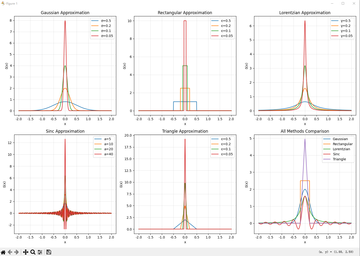
def gaussian_approx(x, sigma):"""高斯函数近似"""return np.exp(-x**2/(2*sigma**2)) / (sigma * np.sqrt(2*np.pi))def rect_approx(x, epsilon):"""矩形函数近似"""return np.where(np.abs(x) <= epsilon, 1/(2*epsilon), 0)def lorentz_approx(x, gamma):"""洛伦兹函数近似"""return gamma / (np.pi * (x**2 + gamma**2))def sinc_approx(x, a):"""sinc函数近似"""return np.sinc(x * a) * a / np.pidef triangle_approx(x, epsilon):"""三角波函数近似"""return np.where(np.abs(x) <= epsilon, (epsilon - np.abs(x))/epsilon**2, 0)# 创建坐标轴
x = np.linspace(-2, 2, 1000)# 1. 展示不同函数的δ函数近似
plt.figure(figsize=(15, 10))# 高斯函数近似
plt.subplot(2, 3, 1)
for sigma in [0.5, 0.2, 0.1, 0.05]:plt.plot(x, gaussian_approx(x, sigma), label=f'σ={sigma}')
plt.title('Gaussian Approximation')
plt.xlabel('x')
plt.ylabel('δ(x)')
plt.legend()
plt.grid(True, alpha=0.3)# 矩形函数近似
plt.subplot(2, 3, 2)
for epsilon in [0.5, 0.2, 0.1, 0.05]:plt.plot(x, rect_approx(x, epsilon), label=f'ε={epsilon}')
plt.title('Rectangular Approximation')
plt.xlabel('x')
plt.ylabel('δ(x)')
plt.legend()
plt.grid(True, alpha=0.3)# 洛伦兹函数近似
plt.subplot(2, 3, 3)
for gamma in [0.5, 0.2, 0.1, 0.05]:plt.plot(x, lorentz_approx(x, gamma), label=f'γ={gamma}')
plt.title('Lorentzian Approximation')
plt.xlabel('x')
plt.ylabel('δ(x)')
plt.legend()
plt.grid(True, alpha=0.3)# sinc函数近似
plt.subplot(2, 3, 4)
for a in [5, 10, 20, 40]:plt.plot(x, sinc_approx(x, a), label=f'a={a}')
plt.title('Sinc Approximation')
plt.xlabel('x')
plt.ylabel('δ(x)')
plt.legend()
plt.grid(True, alpha=0.3)# 三角波函数近似
plt.subplot(2, 3, 5)
for epsilon in [0.5, 0.2, 0.1, 0.05]:plt.plot(x, triangle_approx(x, epsilon), label=f'ε={epsilon}')
plt.title('Triangle Approximation')
plt.xlabel('x')
plt.ylabel('δ(x)')
plt.legend()
plt.grid(True, alpha=0.3)# 所有方法比较(使用相似参数)
plt.subplot(2, 3, 6)
param = 0.2
plt.plot(x, gaussian_approx(x, param), label='Gaussian')
plt.plot(x, rect_approx(x, param), label='Rectangular')
plt.plot(x, lorentz_approx(x, param), label='Lorentzian')
plt.plot(x, sinc_approx(x, 1/param), label='Sinc')
plt.plot(x, triangle_approx(x, param), label='Triangle')
plt.title('All Methods Comparison')
plt.xlabel('x')
plt.ylabel('δ(x)')
plt.legend()
plt.grid(True, alpha=0.3)plt.tight_layout()
plt.show()# 2. 验证筛选性质 (Sampling Property)
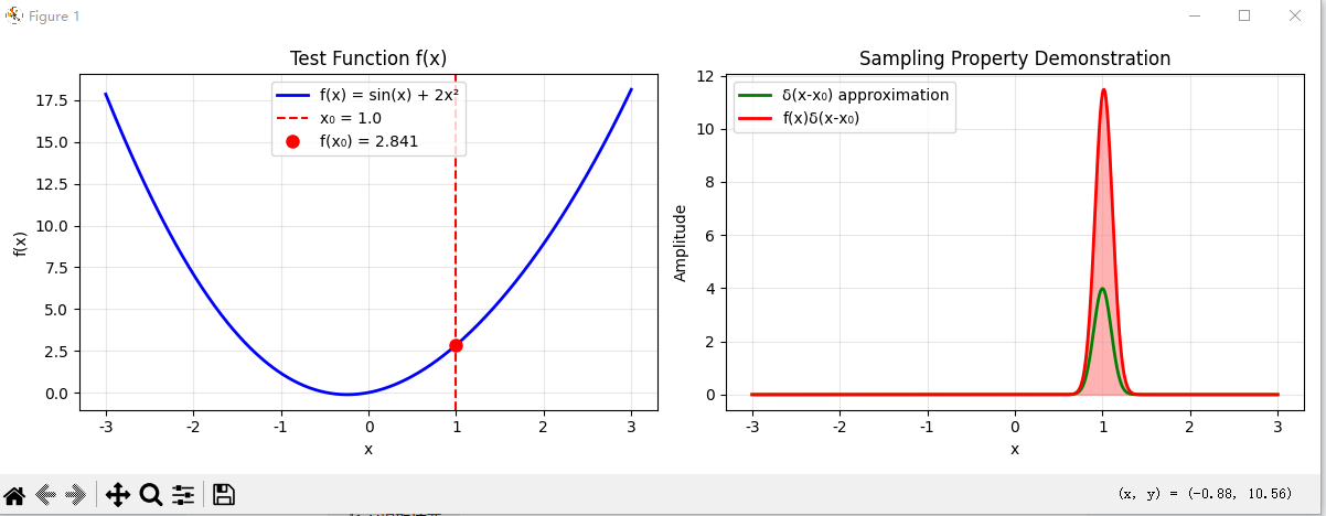
print("验证筛选性质: ∫f(x)δ(x-x₀)dx = f(x₀)")def test_sampling_property():"""测试筛选性质"""# 测试函数def f(x):return np.sin(x) + 2*x**2x0 = 1.0 # 采样点x_range = np.linspace(-3, 3, 1000)dx = x_range[1] - x_range[0]# 使用高斯近似sigma = 0.1delta_approx = gaussian_approx(x_range - x0, sigma)# 计算积分integral = np.sum(f(x_range) * delta_approx) * dxexact_value = f(x0)print(f"数值积分结果: {integral:.6f}")print(f"精确值 f({x0}): {exact_value:.6f}")print(f"相对误差: {abs(integral - exact_value)/abs(exact_value)*100:.4f}%")# 绘图展示plt.figure(figsize=(12, 4))plt.subplot(1, 2, 1)plt.plot(x_range, f(x_range), 'b-', label='f(x) = sin(x) + 2x²', linewidth=2)plt.axvline(x=x0, color='r', linestyle='--', label=f'x₀ = {x0}')plt.plot(x0, exact_value, 'ro', markersize=8, label=f'f(x₀) = {exact_value:.3f}')plt.xlabel('x')plt.ylabel('f(x)')plt.title('Test Function f(x)')plt.legend()plt.grid(True, alpha=0.3)plt.subplot(1, 2, 2)plt.plot(x_range, delta_approx, 'g-', label='δ(x-x₀) approximation', linewidth=2)plt.plot(x_range, f(x_range) * delta_approx, 'r-', label='f(x)δ(x-x₀)', linewidth=2)plt.fill_between(x_range, f(x_range) * delta_approx, alpha=0.3, color='red')plt.xlabel('x')plt.ylabel('Amplitude')plt.title('Sampling Property Demonstration')plt.legend()plt.grid(True, alpha=0.3)plt.tight_layout()plt.show()return integral, exact_valuetest_sampling_property()# 3. 验证缩放性质 (Scaling Property)
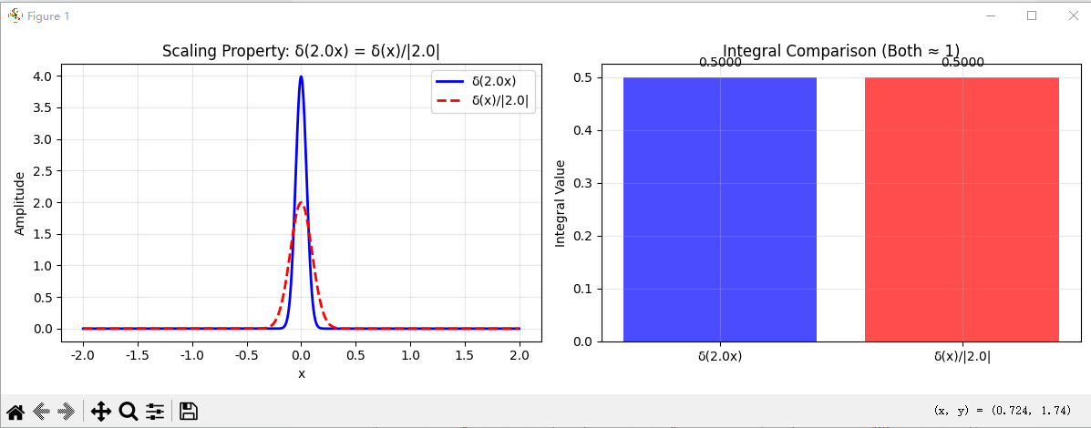
def test_scaling_property():"""测试缩放性质: δ(ax) = δ(x)/|a|"""x = np.linspace(-2, 2, 1000)a = 2.0 # 缩放因子sigma = 0.1# δ(ax)delta_ax = gaussian_approx(a * x, sigma)# δ(x)/|a|delta_scaled = gaussian_approx(x, sigma) / abs(a)plt.figure(figsize=(12, 4))plt.subplot(1, 2, 1)plt.plot(x, delta_ax, 'b-', label=f'δ({a}x)', linewidth=2)plt.plot(x, delta_scaled, 'r--', label=f'δ(x)/|{a}|', linewidth=2)plt.xlabel('x')plt.ylabel('Amplitude')plt.title(f'Scaling Property: δ({a}x) = δ(x)/|{a}|')plt.legend()plt.grid(True, alpha=0.3)# 验证积分相等dx = x[1] - x[0]integral_ax = np.sum(delta_ax) * dxintegral_scaled = np.sum(delta_scaled) * dxplt.subplot(1, 2, 2)methods = [f'δ({a}x)', f'δ(x)/|{a}|']integrals = [integral_ax, integral_scaled]plt.bar(methods, integrals, color=['blue', 'red'], alpha=0.7)plt.ylabel('Integral Value')plt.title('Integral Comparison (Both ≈ 1)')plt.grid(True, alpha=0.3)for i, v in enumerate(integrals):plt.text(i, v + 0.02, f'{v:.4f}', ha='center')plt.tight_layout()plt.show()print(f"缩放性质验证:")print(f"∫δ({a}x)dx = {integral_ax:.6f}")print(f"∫[δ(x)/|{a}|]dx = {integral_scaled:.6f}")test_scaling_property()# 4. 验证偶函数性质 (Even Function Property)
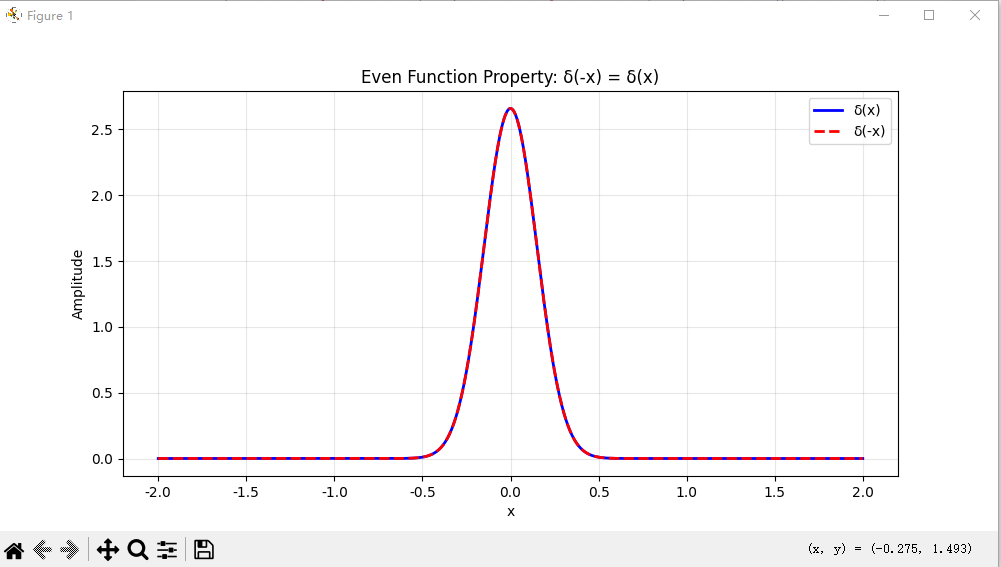
def test_even_property():"""测试偶函数性质: δ(-x) = δ(x)"""x = np.linspace(-2, 2, 1000)sigma = 0.15delta_x = gaussian_approx(x, sigma)delta_minus_x = gaussian_approx(-x, sigma)plt.figure(figsize=(10, 5))plt.plot(x, delta_x, 'b-', label='δ(x)', linewidth=2)plt.plot(x, delta_minus_x, 'r--', label='δ(-x)', linewidth=2)plt.xlabel('x')plt.ylabel('Amplitude')plt.title('Even Function Property: δ(-x) = δ(x)')plt.legend()plt.grid(True, alpha=0.3)# 计算最大差异max_diff = np.max(np.abs(delta_x - delta_minus_x))print(f"偶函数性质验证:")print(f"δ(x) 和 δ(-x) 的最大差异: {max_diff:.6e} (应该接近0)")plt.show()test_even_property()# 5. 验证复合函数性质
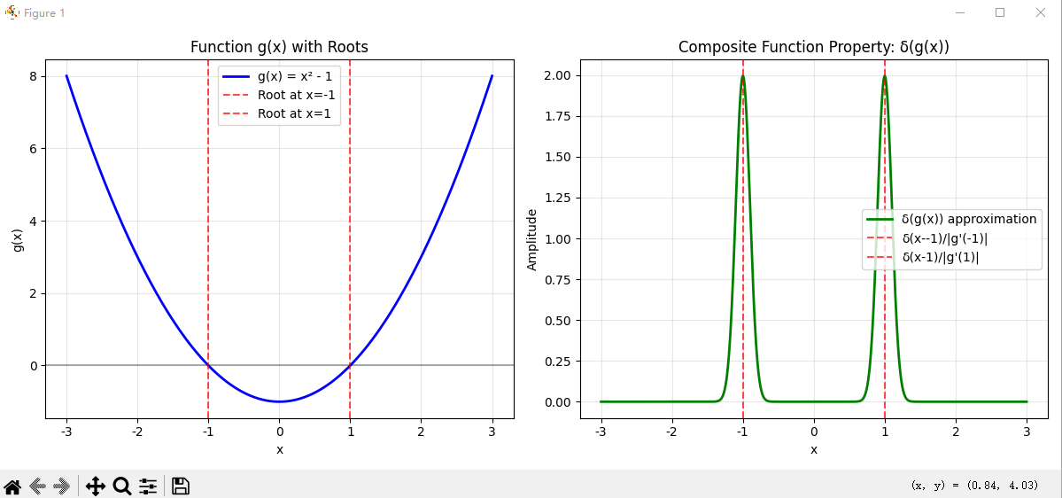
def test_composite_property():"""测试复合函数性质: δ(g(x))"""x = np.linspace(-3, 3, 1000)# 定义 g(x) = x² - 1,根在 x = ±1def g(x):return x**2 - 1# 使用性质: δ(g(x)) = Σ δ(x-xᵢ)/|g'(xᵢ)|roots = [-1, 1] # g(x) = 0 的根derivatives = [abs(2*root) for root in roots] # |g'(xᵢ)|sigma = 0.1delta_composite = np.zeros_like(x)for root, deriv in zip(roots, derivatives):delta_composite += gaussian_approx(x - root, sigma) / derivplt.figure(figsize=(12, 5))plt.subplot(1, 2, 1)plt.plot(x, g(x), 'b-', label='g(x) = x² - 1', linewidth=2)plt.axhline(y=0, color='k', linestyle='-', alpha=0.3)for root in roots:plt.axvline(x=root, color='r', linestyle='--', alpha=0.7, label=f'Root at x={root}')plt.xlabel('x')plt.ylabel('g(x)')plt.title('Function g(x) with Roots')plt.legend()plt.grid(True, alpha=0.3)plt.subplot(1, 2, 2)plt.plot(x, delta_composite, 'g-', label='δ(g(x)) approximation', linewidth=2)for root, deriv in zip(roots, derivatives):plt.axvline(x=root, color='r', linestyle='--', alpha=0.7, label=f'δ(x-{root})/|g\'({root})|')plt.xlabel('x')plt.ylabel('Amplitude')plt.title('Composite Function Property: δ(g(x))')plt.legend()plt.grid(True, alpha=0.3)plt.tight_layout()plt.show()test_composite_property()# 6. 验证卷积性质 (Convolution Property)
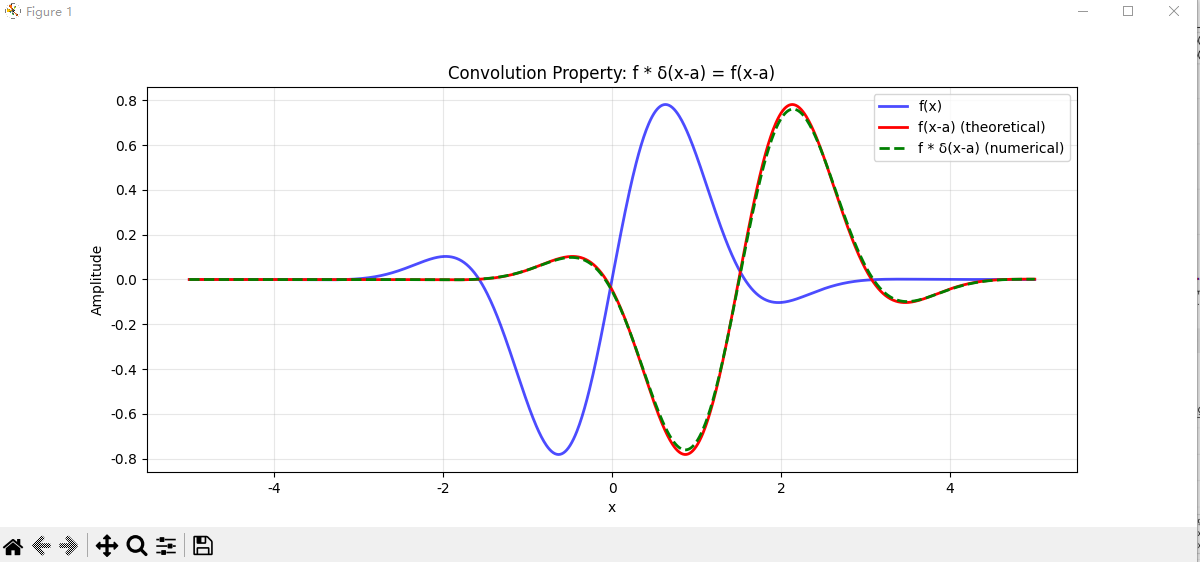
def test_convolution_property():"""测试卷积性质: f * δ(x-a) = f(x-a)"""x = np.linspace(-5, 5, 1000)dx = x[1] - x[0]# 测试函数def f(x):return np.exp(-x**2/2) * np.sin(2*x)a = 1.5 # 平移量sigma = 0.1# δ(x-a)delta_shifted = gaussian_approx(x - a, sigma)# 数值卷积convolution = np.convolve(f(x), delta_shifted, mode='same') * dx# 理论结果: f(x-a)theoretical = f(x - a)plt.figure(figsize=(12, 5))plt.plot(x, f(x), 'b-', label='f(x)', linewidth=2, alpha=0.7)plt.plot(x, theoretical, 'r-', label='f(x-a) (theoretical)', linewidth=2)plt.plot(x, convolution, 'g--', label='f * δ(x-a) (numerical)', linewidth=2)plt.xlabel('x')plt.ylabel('Amplitude')plt.title('Convolution Property: f * δ(x-a) = f(x-a)')plt.legend()plt.grid(True, alpha=0.3)# 计算误差error = np.max(np.abs(convolution - theoretical))print(f"卷积性质验证:")print(f"最大误差: {error:.6f}")plt.show()test_convolution_property()# 7. 总结:所有近似的积分验证
print("\n" + "="*50)
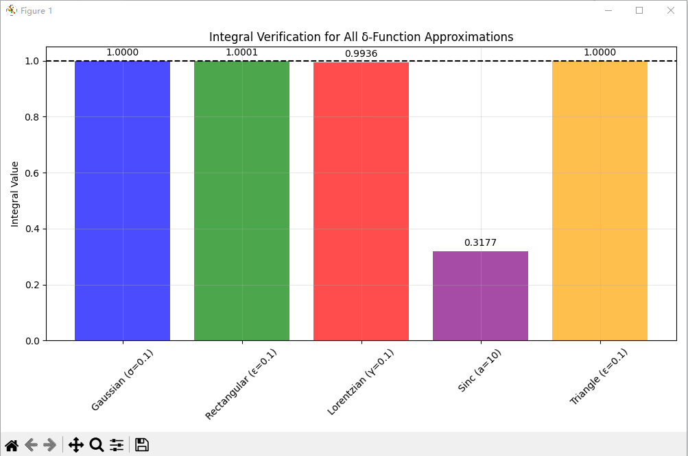
print("所有δ函数近似的积分验证 (应该都接近1)")
print("="*50)x_test = np.linspace(-10, 10, 10000)
dx_test = x_test[1] - x_test[0]methods = {'Gaussian (σ=0.1)': gaussian_approx(x_test, 0.1),'Rectangular (ε=0.1)': rect_approx(x_test, 0.1),'Lorentzian (γ=0.1)': lorentz_approx(x_test, 0.1),'Sinc (a=10)': sinc_approx(x_test, 10),'Triangle (ε=0.1)': triangle_approx(x_test, 0.1)
}plt.figure(figsize=(10, 6))
integrals = []
names = []for name, approx in methods.items():integral = np.sum(approx) * dx_testintegrals.append(integral)names.append(name)print(f"{name:20s}: {integral:.6f}")plt.bar(names, integrals, color=['blue', 'green', 'red', 'purple', 'orange'], alpha=0.7)
plt.axhline(y=1, color='k', linestyle='--', label='Theoretical value: 1')
plt.ylabel('Integral Value')
plt.title('Integral Verification for All δ-Function Approximations')
plt.xticks(rotation=45)
plt.grid(True, alpha=0.3)for i, v in enumerate(integrals):plt.text(i, v + 0.02, f'{v:.4f}', ha='center')plt.tight_layout()
plt.show()