Halcon卡尺 Measure_pos原理与实现（C++ 和Python版本，基于OpenCV）

一、原理介绍

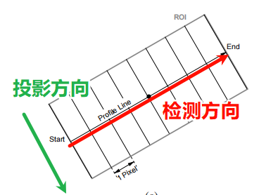
Measure_pos算子功能：提取垂直于矩形或环形弧的直边。
原理：

1.1 灰度平均

垂直于检测线方向（投影方向），在指定宽度下做灰度平均。
关键：插值方法

1.2 灰度剖面线平滑

对灰度平均后的灰度剖面线进行高斯滤波进行平滑
关键：高斯滤波 （size=3sigma+1）

1.3 灰度剖面线求导

对平滑后的灰度剖面线求高斯一阶导数。
关键：高斯滤波（size=3sigma+1,sigma=0.4）

1.4 查找边缘

设定导数阈值T,将大于T和小于-T的部分进行二次曲线拟合找到极值位置

二、代码实现

2.1测试图像

2.2 c++代码

#include <opencv2/opencv.hpp>
#include <iostream>
#include <vector>
#include <numeric>
#include<fstream>struct EdgePoint
{double position;  // 亚像素位置int polarity;     // +1 黑->白, -1 白->黑float gradient;   // 最大梯度值
};// 二次曲线拟合亚像素极值
double fitQuadraticSubpixel(const std::vector<float>& x, const std::vector<float>& y)
{int n = static_cast<int>(x.size());if (n < 3) return x[n / 2];// 1. 居中平移 x，避免数值漂移double x_mean = std::accumulate(x.begin(), x.end(), 0.0) / n;std::vector<double> xs(n);for (int i = 0; i < n; ++i)xs[i] = x[i] - x_mean;// 2. 计算矩阵项double sumX = 0, sumX2 = 0, sumX3 = 0, sumX4 = 0;double sumY = 0, sumXY = 0, sumX2Y = 0;for (int i = 0; i < n; ++i){double xi = xs[i];double yi = y[i];double xi2 = xi * xi;sumX += xi;sumX2 += xi2;sumX3 += xi2 * xi;sumX4 += xi2 * xi2;sumY += yi;sumXY += xi * yi;sumX2Y += xi2 * yi;}cv::Mat A = (cv::Mat_<double>(3, 3) << sumX4, sumX3, sumX2,sumX3, sumX2, sumX,sumX2, sumX, n);cv::Mat B = (cv::Mat_<double>(3, 1) << sumX2Y, sumXY, sumY);cv::Mat coeff;cv::solve(A, B, coeff, cv::DECOMP_SVD);double a = coeff.at<double>(0);double b = coeff.at<double>(1);if (std::abs(a) < 1e-8) return x[n / 2];// 3. 求极值位置（局部坐标）double x_peak_local = -b / (2 * a);// 4. 还原全局坐标double x_peak = x_peak_local + x_mean;// 5. 保证在范围内if (x_peak < x.front()) x_peak = x.front();if (x_peak > x.back())  x_peak = x.back();return x_peak;
}// 双线性插值读取灰度（单通道 CV_8U），超出边界时使用边界复制
static inline float sampleBilinear(const cv::Mat& img, double x, double y) {int w = img.cols, h = img.rows;if (x < 0) x = 0;if (y < 0) y = 0;if (x > w - 1) x = w - 1;if (y > h - 1) y = h - 1;int x0 = (int)std::floor(x);int y0 = (int)std::floor(y);int x1 = std::min(x0 + 1, w - 1);int y1 = std::min(y0 + 1, h - 1);double dx = x - x0;double dy = y - y0;float I00 = img.at<uchar>(y0, x0);float I10 = img.at<uchar>(y0, x1);float I01 = img.at<uchar>(y1, x0);float I11 = img.at<uchar>(y1, x1);double I = (1 - dx) * (1 - dy) * I00 + dx * (1 - dy) * I10 + (1 - dx) * dy * I01 + dx * dy * I11;return (float)I;
}cv::Mat detectEdgesAlongLine(const cv::Mat& gray,const cv::Point2f& p1,const cv::Point2f& p2,int width,int sigma) {CV_Assert(!gray.empty() && gray.type() == CV_8U);if (width <= 0) width = 3;cv::Point2f v = p2 - p1;double length = std::hypot(v.x, v.y);if (length < 1.0) return {};cv::Point2f u = v * (1.0f / (float)length);cv::Point2f perp(-u.y, u.x);std::vector<float> profile; profile.reserve(length);int halfW = width / 2;for (int i = 0; i < length; ++i) {double t = (double)i;cv::Point2f center = p1 + u * (float)t;double sum = 0.0;for (int k = -halfW; k <= halfW; ++k) {cv::Point2f samplePt = center + perp * (float)k;float val = sampleBilinear(gray, samplePt.x, samplePt.y);sum += val;}float avg = (float)(sum / (double)(2 * halfW + 1));profile.push_back(avg);}cv::Mat profMat(profile);cv::Mat profF;profMat.convertTo(profF, CV_32F);cv::Mat profRow = profF.t();int smooth_ksize = 6 * sigma + 1;cv::GaussianBlur(profRow, profRow, cv::Size(smooth_ksize, 1), 0, 0, cv::BORDER_REPLICATE);return profRow.t();
}// 生成高斯导数核 G'(x)
static std::vector<float> makeGaussianDerivativeKernel(double sigma)
{int radius = static_cast<int>(std::ceil(3 * sigma));  // 截断范围 ±3σint size = 2 * radius + 1;std::vector<float> kernel(size);double sigma2 = sigma * sigma;double norm = 0.0;for (int i = -radius; i <= radius; ++i){// 高斯一阶导数公式：G'(x) = -(x / σ²) * exp(-x² / (2σ²))double val = -(i / sigma2) * std::exp(-0.5 * (i * i) / sigma2);kernel[i + radius] = static_cast<float>(val);norm += std::abs(val);}// 归一化（可选），只保证尺度一致，不影响梯度位置if (norm > 0){for (auto& v : kernel) v /= static_cast<float>(norm);}return kernel;
}// 一维卷积
static std::vector<float> convolve1D(const std::vector<float>& signal, const std::vector<float>& kernel)
{int half = static_cast<int>(kernel.size() / 2);std::vector<float> result(signal.size(), 0.0f);for (size_t i = 0; i < signal.size(); ++i){double sum = 0.0;for (int k = -half; k <= half; ++k){int idx = static_cast<int>(i) + k;if (idx < 0) idx = 0;if (idx >= static_cast<int>(signal.size())) idx = static_cast<int>(signal.size()) - 1;sum += signal[idx] * kernel[half - k];}result[i] = static_cast<float>(sum);}return result;
}//计算剖面的一阶导数
std::vector<float> computeProfileGradient(const std::vector<float>& profile, double sigma = 1.0)
{if (profile.empty())return {};// 1. 生成高斯一阶导核auto kernel = makeGaussianDerivativeKernel(sigma);// 2. 卷积求导数auto grad = convolve1D(profile, kernel);// 3. 恢复尺度for (auto& v : grad) v *= sigma * std::sqrt(2.0 * CV_PI);return grad;
}std::vector<EdgePoint> findAllEdgesPeak(const std::vector<float>derivProfile, double threshold)
{std::vector<EdgePoint> edges;cv::Mat profile;int n = derivProfile.size();int start = -1;// 3. 找超过阈值的连续区段for (int i = 0; i < n - 1; ++i){if (std::abs(derivProfile[i]) > threshold){if (start == -1)start = i;}else if (start != -1){int end = i - 1;// 4. 寻找区段内梯度极值点float maxVal = 0;int maxIdx = start;for (int j = start; j <= end; ++j){if (std::abs(derivProfile[j]) > std::abs(maxVal)){maxVal = derivProfile[j];maxIdx = j;}}// 5. 在极值点附近（±2）取窗口做最小二乘拟合std::vector<float> x, y;for (int k = maxIdx - 2; k <= maxIdx + 2; ++k){if (k >= 0 && k < n - 1){x.push_back((float)k);y.push_back(derivProfile[k]);}}double subPos = fitQuadraticSubpixel(x, y) + 0.5;int polarity = (maxVal > 0) ? +1 : -1;edges.push_back({ subPos, polarity, maxVal });start = -1;}}return edges;
}// 保存参数到本地文件
template< typename T>
void savePara(std::string path, std::vector<T>para)
{std::ofstream out(path);for(auto v : para){out << v << ",";}out.close();
}int main()
{/** 图像边缘检测相关代码示例* 该代码段主要实现了沿直线检测图像边缘的功能*/// 读取灰度图像cv::Mat img = cv::imread("C:/Users/z126w/Desktop/1.png", cv::IMREAD_GRAYSCALE);//用于显示cv::Mat displayImg;cv::cvtColor(img.clone(), displayImg, cv::COLOR_GRAY2BGR);// 检查图像是否成功加载if (img.empty()) {// 如果图像加载失败，输出错误信息并返回-1std::cerr << "Cannot open image\n";return -1;}// 定义直线的起点和终点坐标cv::Point2f p1(0, img.rows / 2), p2(img.cols, img.rows / 2);// 设置参数int width = img.rows / 2;          // 线的宽度double deriv_thresh = 8.0;  // 导数阈值int sigma = 1;          // 高斯滤波的标准差// 沿直线检测边缘auto grayProfile = detectEdgesAlongLine(img, p1, p2, width, sigma);//保存本地测试savePara<float>("grayProfile.txt", grayProfile);//2.高斯求导auto derivProfile = computeProfileGradient(grayProfile, 0.4);savePara<float>("derivProfile.txt", derivProfile);// 查找所有边缘峰值auto edges = findAllEdgesPeak(derivProfile, deriv_thresh);for (const auto& edge : edges) {cv::Point2f v = p2 - p1;double length = std::hypot(v.x, v.y);cv::Point2f u = v * (1.0f / (float)length);cv::Point2f perp(-u.y, u.x);auto linePoint = edge.position * u + p1;auto start = linePoint + perp * (width / 2);auto end = linePoint - perp * (width / 2);cv::line(displayImg, start, end, cv::Scalar(0, 0, 255), 1, cv::LINE_AA);}cv::imshow("Detected Edges", displayImg);// 程序正常结束，返回0return 0;
}

2.3对比halcon验证

2.3.1 halcon实现代码

read_image (Image1, 'C:/Users/z126w/Desktop/1.png')
gray_projections (Image1, Image1, 'simple', HorProjection, VertProjection)
create_funct_1d_array (VertProjection, Function)
smooth_funct_1d_gauss (Function, 1, SmoothedFunction)
derivate_funct_1d (SmoothedFunction, 'first', Derivative)
funct_1d_to_pairs (Derivative, XValues, YValues)*对比测试
open_file ('C:/Users/z126w/source/repos/testCodeAccelerate/testCodeAccelerate/grayProfile.txt', 'input', FileHandle)
fread_line (FileHandle, OutLine, IsEOF)
tuple_split (OutLine, ',', Substrings)
tuple_number (Substrings, grayProfile)open_file ('C:/Users/z126w/source/repos/testCodeAccelerate/testCodeAccelerate/derivProfile.txt', 'input', gradFileHandle)
fread_line (gradFileHandle, OutLine1, IsEOF)
tuple_split (OutLine1, ',', Substrings1)
tuple_number (Substrings1, gradProfile)

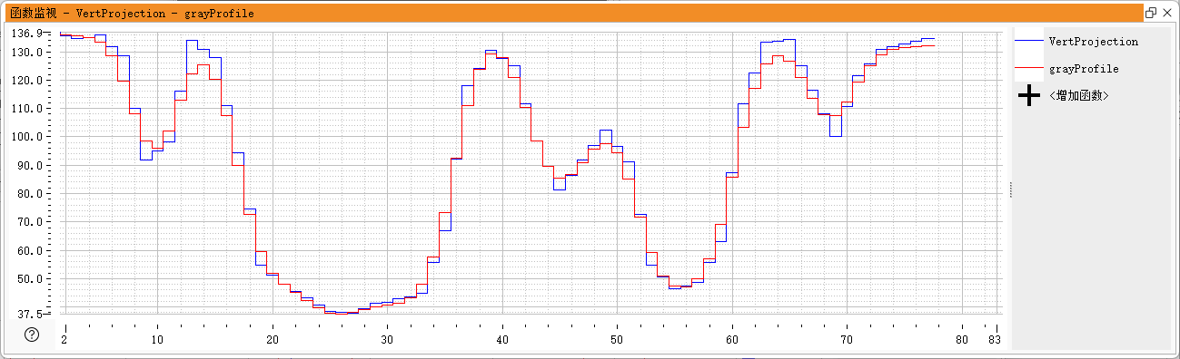
2.3.2 灰度平均对比

图像红色为我们，蓝色为halcon

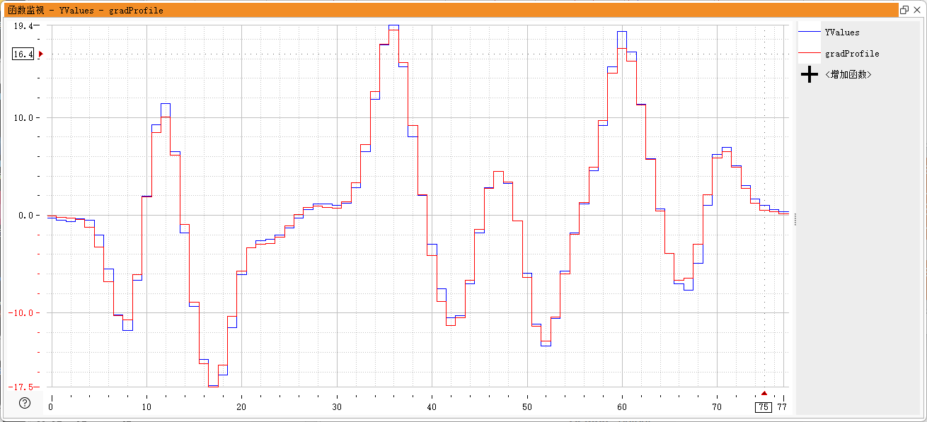
2.3.3 导数对比

图像红色为我们，蓝色为halcon

2.4 python版本

import cv2
import numpy as np
import matplotlib.pyplot as plt
import math
import scipy.ndimage as ndiimage = cv2.imread('image.png')
gray = cv2.cvtColor(image, cv2.COLOR_BGR2GRAY)
f = np.float32(gray)
profile = cv2.reduce(f, 0, cv2.REDUCE_AVG)xAxis = np.array(range(len(profile[0])))
plt.plot(xAxis, profile[0])
plt.show()edge = ndi.gaussian_filter(profile,sigma=0.4,order=[0,1],output=np.float64, mode='nearest')
edge = edge * math.sqrt(2 * math.pi)
plt.plot(xAxis, edge[0])
plt.show()