「用Python来学微积分」14. 连续函数的运算与初等函数的连续性
一、连续函数的四则运算
定理2 如果函数 f(x) 和 g(x) 均在 x₀ 处连续,那么它们的和、差、积、商函数 f(x)±g(x),f(x)g(x),f(x)/g(x)(g(x₀)≠0)均在 x₀ 处连续。
下面通过Python可视化来直观理解这个定理:
import matplotlib.pyplot as plt
import numpy as npdef demonstrate_continuous_operations():x = np.linspace(-2, 2, 1000)# 定义两个连续函数f = lambda x: np.sin(x)  # 连续函数g = lambda x: x**2 + 1   # 连续函数# 计算各种运算结果f_plus_g = f(x) + g(x)   # 和函数f_minus_g = f(x) - g(x)  # 差函数f_times_g = f(x) * g(x)  # 积函数f_div_g = f(x) / g(x)    # 商函数(g(x) ≠ 0)fig, axes = plt.subplots(2, 3, figsize=(15, 10))# 原始函数axes[0,0].plot(x, f(x), 'b-', linewidth=2, label='f(x) = sin(x)')axes[0,0].set_title('连续函数 f(x)')axes[0,0].grid(True)axes[0,0].legend()axes[0,1].plot(x, g(x), 'r-', linewidth=2, label='g(x) = x² + 1')axes[0,1].set_title('连续函数 g(x)')axes[0,1].grid(True)axes[0,1].legend()# 四则运算结果axes[0,2].plot(x, f_plus_g, 'g-', linewidth=2, label='f(x) + g(x)')axes[0,2].set_title('和函数: f(x) + g(x)')axes[0,2].grid(True)axes[0,2].legend()axes[1,0].plot(x, f_minus_g, 'purple', linewidth=2, label='f(x) - g(x)')axes[1,0].set_title('差函数: f(x) - g(x)')axes[1,0].grid(True)axes[1,0].legend()axes[1,1].plot(x, f_times_g, 'orange', linewidth=2, label='f(x) × g(x)')axes[1,1].set_title('积函数: f(x) × g(x)')axes[1,1].grid(True)axes[1,1].legend()# 商函数(注意去除g(x)=0的点)mask = g(x) != 0axes[1,2].plot(x[mask], f_div_g[mask], 'brown', linewidth=2, label='f(x) / g(x)')axes[1,2].set_title('商函数: f(x) / g(x)')axes[1,2].grid(True)axes[1,2].legend()plt.tight_layout()plt.show()# 验证在x=0处的连续性x0 = 0print(f"在 x = {x0} 处:")print(f"f({x0}) = {f(x0):.6f}, g({x0}) = {g(x0):.6f}")print(f"f+g({x0}) = {f(x0) + g(x0):.6f}")print(f"f-g({x0}) = {f(x0) - g(x0):.6f}")print(f"f×g({x0}) = {f(x0) * g(x0):.6f}")print(f"f/g({x0}) = {f(x0) / g(x0):.6f}")demonstrate_continuous_operations()
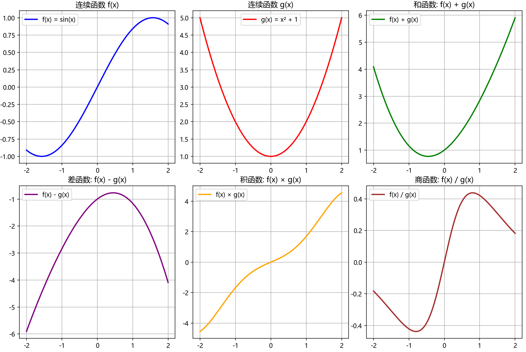
运行结果分析: 从图像可以看出,两个连续函数的和、差、积、商(分母不为零时)仍然是连续函数,验证了定理2的正确性。
二、复合函数的连续性
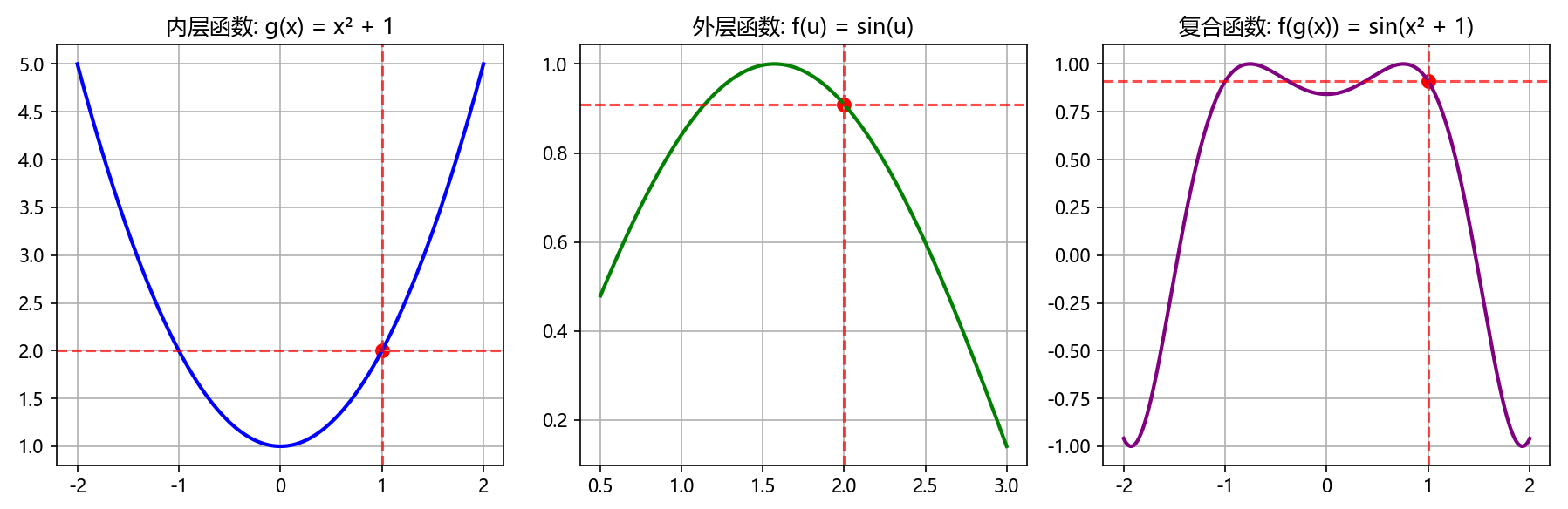
定理3 如果函数 f(u) 在 u₀ 处连续,函数 g(x) 在 x₀ 处连续,且 u₀ = g(x₀),那么复合函数 f(g(x)) 在 x₀ 处连续。
从运算的角度看,在定理3的条件下,有: limx→x0f(g(x))=f(limx→x0g(x))=f(g(limx→x0x))\lim_{x \to x_0} f(g(x)) = f(\lim_{x \to x_0} g(x)) = f(g(\lim_{x \to x_0} x))x→x0limf(g(x))=f(x→x0limg(x))=f(g(x→x0limx)) 成立,即对连续函数来说,极限求值运算与函数求值运算可以交换次序。
import matplotlib.pyplot as plt
import numpy as np# 设置支持 Unicode 的字体
plt.rcParams['font.sans-serif'] = ['Microsoft YaHei','DejaVu Sans']
plt.rcParams['axes.unicode_minus'] = Falsedef demonstrate_composite_continuity():x = np.linspace(-2, 2, 1000)# 内层函数g = lambda x: x**2 + 1# 外层函数f = lambda u: np.sin(u)# 复合函数fog = lambda x: f(g(x))# 验证在x=1处的连续性x0 = 1u0 = g(x0)print("复合函数连续性验证:")print(f"x₀ = {x0}, g(x₀) = {u0:.6f}, f(g(x₀)) = {fog(x0):.6f}")print(f"lim(x→{x0}) g(x) = {g(x0):.6f}")print(f"lim(u→{u0}) f(u) = {f(u0):.6f}")print(f"lim(x→{x0}) f(g(x)) = {fog(x0):.6f}")print("由于 f(g(x₀)) = lim(x→x₀) f(g(x)),复合函数在 x₀ 处连续")# 绘制图像plt.figure(figsize=(12, 4))plt.subplot(1, 3, 1)plt.plot(x, g(x), 'b-', linewidth=2)plt.axvline(x=x0, color='r', linestyle='--', alpha=0.7)plt.axhline(y=u0, color='r', linestyle='--', alpha=0.7)plt.scatter([x0], [u0], color='red', s=50)plt.title('内层函数: g(x) = x² + 1')plt.grid(True)plt.subplot(1, 3, 2)u_values = np.linspace(0.5, 3, 1000)plt.plot(u_values, f(u_values), 'g-', linewidth=2)plt.axvline(x=u0, color='r', linestyle='--', alpha=0.7)plt.axhline(y=f(u0), color='r', linestyle='--', alpha=0.7)plt.scatter([u0], [f(u0)], color='red', s=50)plt.title('外层函数: f(u) = sin(u)')plt.grid(True)plt.subplot(1, 3, 3)plt.plot(x, fog(x), 'purple', linewidth=2)plt.axvline(x=x0, color='r', linestyle='--', alpha=0.7)plt.axhline(y=fog(x0), color='r', linestyle='--', alpha=0.7)plt.scatter([x0], [fog(x0)], color='red', s=50)plt.title('复合函数: f(g(x)) = sin(x² + 1)')plt.grid(True)plt.tight_layout()plt.show()demonstrate_composite_continuity()
三、初等函数的连续性证明
例1:幂函数的连续性证明
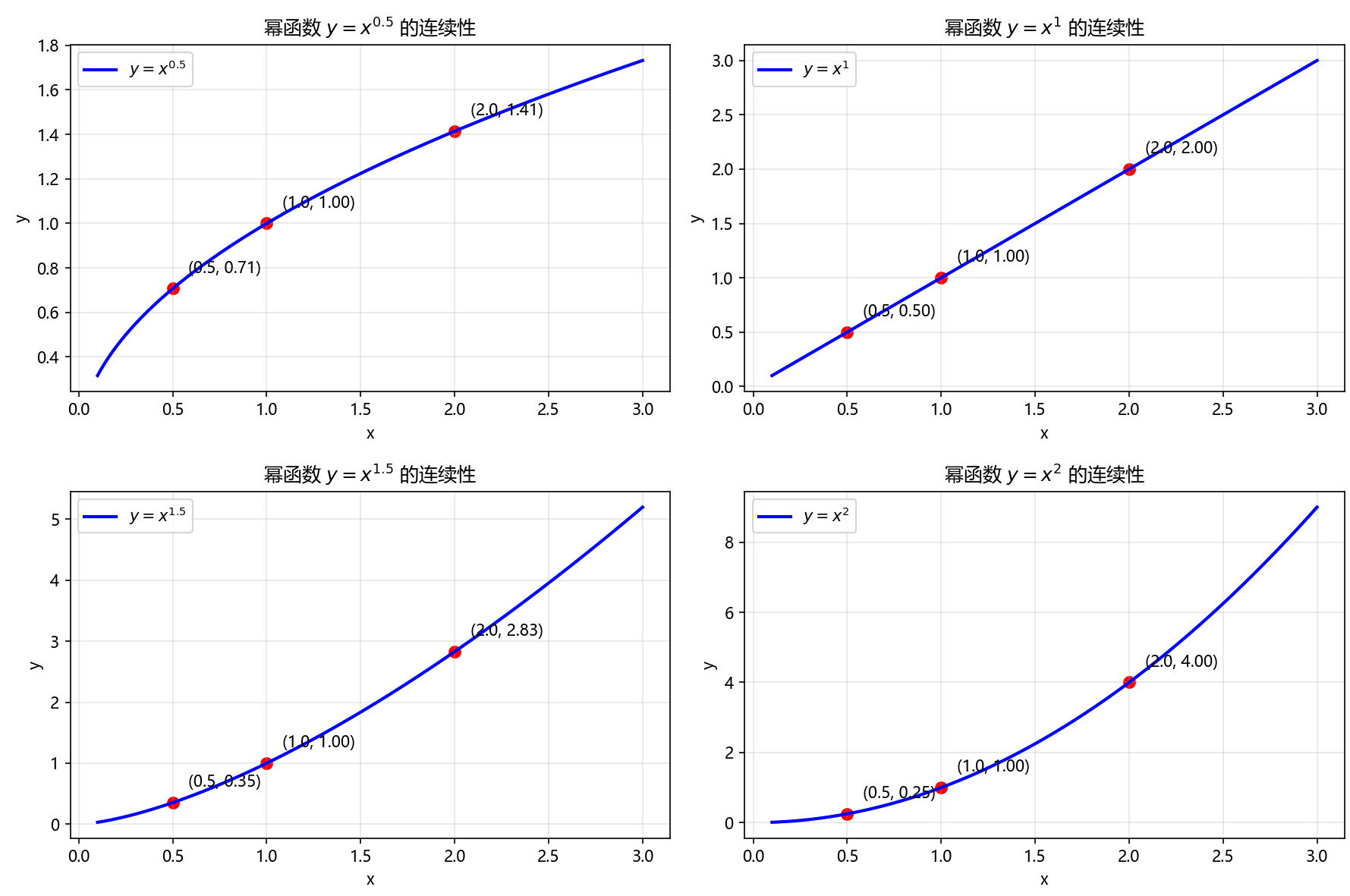
证明:幂函数 y=xαy = x^\alphay=xα 在 (0,+∞)(0, +\infty)(0,+∞) 内连续。
证明过程:当 x∈(0,+∞)x \in (0, +\infty)x∈(0,+∞) 时,根据指数函数与对数函数的性质,得: y=xα=elnxα=eαlnxy = x^\alpha = e^{\ln x^\alpha} = e^{\alpha \ln x}y=xα=elnxα=eαlnx
由于对数函数与指数函数都是连续的,因此对任意的 x0∈(0,+∞)x_0 \in (0, +\infty)x0∈(0,+∞),因为函数 αlnx\alpha \ln xαlnx 在 x0x_0x0 处连续,且指数函数 exe^xex 在 u0=αlnx0u_0 = \alpha \ln x_0u0=αlnx0 处连续,所以根据复合函数的连续性可知,幂函数 y=xα=eαlnxy = x^\alpha = e^{\alpha \ln x}y=xα=eαlnx 在 x0x_0x0 处连续。
由 x0x_0x0 的任意性可知:幂函数 y=xαy = x^\alphay=xα 在 (0,+∞)(0, +\infty)(0,+∞) 内连续。
def demonstrate_power_function_continuity():x = np.linspace(0.1, 3, 1000)alpha_values = [0.5, 1, 1.5, 2] # 不同的指数plt.figure(figsize=(12, 8))for i, alpha in enumerate(alpha_values):y = x**alphaplt.subplot(2, 2, i+1)plt.plot(x, y, 'b-', linewidth=2, label=f'$y = x^{{{alpha}}}$')# 标记几个点验证连续性test_points = [0.5, 1.0, 2.0]for x0 in test_points:y0 = x0**alphaplt.scatter([x0], [y0], color='red', s=50)plt.annotate(f'({x0}, {y0:.2f})', (x0, y0), xytext=(10, 10), textcoords='offset points')plt.title(f'幂函数 $y = x^{{{alpha}}}$ 的连续性')plt.xlabel('x')plt.ylabel('y')plt.grid(True, alpha=0.3)plt.legend()plt.tight_layout()plt.show()# 验证极限运算x0 = 2for alpha in alpha_values:limit_left = (x0 - 0.001)**alphalimit_right = (x0 + 0.001)**alphaactual_value = x0**alphaprint(f"幂函数 y = x^{alpha}:")print(f" lim(x→{x0}-) y = {limit_left:.6f}")print(f" lim(x→{x0}+) y = {limit_right:.6f}")print(f" y({x0}) = {actual_value:.6f}")print(f" 连续性验证: {abs(limit_left - actual_value) < 1e-5 and abs(limit_right - actual_value) < 1e-5}")print()demonstrate_power_function_continuity()
例2:指数型复合函数的连续性
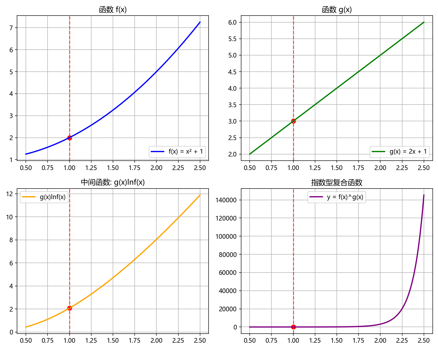
证明:如果函数 f(x) 和 g(x) 均在 x₀ 处连续,且 f(x₀) > 0,则函数 y=f(x)g(x)y = f(x)^{g(x)}y=f(x)g(x) 在 x₀ 处连续。
证明过程:根据指数函数与对数函数的性质,得: y=f(x)g(x)=elnf(x)g(x)=eg(x)lnf(x)y = f(x)^{g(x)} = e^{\ln f(x)^{g(x)}} = e^{g(x) \ln f(x)}y=f(x)g(x)=elnf(x)g(x)=eg(x)lnf(x)
因为函数 f(x) 在 x₀ 处连续,对数函数 lnu\ln ulnu 在 f(x₀) 处连续,所以函数 lnf(x)\ln f(x)lnf(x) 在 x₀ 处连续。
因为函数 g(x) 在 x₀ 处连续,所以函数 g(x)lnf(x)g(x) \ln f(x)g(x)lnf(x) 在 x₀ 处连续。
又因为指数函数 exe^xex 在 v0=g(x0)lnf(x0)v_0 = g(x₀) \ln f(x₀)v0=g(x0)lnf(x0) 处连续,所以 y=eg(x)lnf(x)y = e^{g(x) \ln f(x)}y=eg(x)lnf(x) 在 x₀ 处连续。
import matplotlib.pyplot as plt
import numpy as np# 设置支持 Unicode 的字体
plt.rcParams['font.sans-serif'] = ['Microsoft YaHei', 'DejaVu Sans']
plt.rcParams['axes.unicode_minus'] = Falsedef demonstrate_exponential_composite_continuity():x = np.linspace(0.5, 2.5, 1000)# 定义f(x)和g(x),在x=1处都连续f = lambda x: x**2 + 1  # f(1) = 2 > 0g = lambda x: 2*x + 1# 指数型复合函数y = f(x)**g(x)# 验证在x=1处的连续性x0 = 1f_x0 = f(x0)g_x0 = g(x0)y_x0 = f_x0**g_x0print("指数型复合函数连续性验证:")print(f"在 x = {x0} 处:")print(f"f({x0}) = {f_x0} > 0")print(f"g({x0}) = {g_x0}")# 修复这里:使用g(x0)而不是g({x0})print(f"y({x0}) = f({x0})^{g(x0)} = {y_x0:.6f}")# 计算左右极限x_left = x0 - 0.001x_right = x0 + 0.001y_left = f(x_left)**g(x_left)y_right = f(x_right)**g(x_right)print(f"lim(x→{x0}-) y = {y_left:.6f}")print(f"lim(x→{x0}+) y = {y_right:.6f}")print(f"连续性成立: {abs(y_left - y_x0) < 1e-4 and abs(y_right - y_x0) < 1e-4}")# 绘制图像plt.figure(figsize=(10, 8))plt.subplot(2, 2, 1)plt.plot(x, f(x), 'b-', linewidth=2, label='f(x) = x² + 1')plt.axvline(x=x0, color='r', linestyle='--', alpha=0.7)plt.scatter([x0], [f_x0], color='red', s=50)plt.title('函数 f(x)')plt.grid(True)plt.legend()plt.subplot(2, 2, 2)plt.plot(x, g(x), 'g-', linewidth=2, label='g(x) = 2x + 1')plt.axvline(x=x0, color='r', linestyle='--', alpha=0.7)plt.scatter([x0], [g_x0], color='red', s=50)plt.title('函数 g(x)')plt.grid(True)plt.legend()plt.subplot(2, 2, 3)# 使用对数变换避免数值问题log_y = g(x) * np.log(f(x))plt.plot(x, log_y, 'orange', linewidth=2, label='g(x)lnf(x)')plt.axvline(x=x0, color='r', linestyle='--', alpha=0.7)plt.scatter([x0], [g_x0 * np.log(f_x0)], color='red', s=50)plt.title('中间函数: g(x)lnf(x)')plt.grid(True)plt.legend()plt.subplot(2, 2, 4)plt.plot(x, y, 'purple', linewidth=2, label='y = f(x)^g(x)')plt.axvline(x=x0, color='r', linestyle='--', alpha=0.7)plt.scatter([x0], [y_x0], color='red', s=50)plt.title('指数型复合函数')plt.grid(True)plt.legend()plt.tight_layout()plt.show()# 调用函数
demonstrate_exponential_composite_continuity()
四、初等函数连续性总结
基于前面的证明,我们可以总结出以下重要结论:
- 基本初等函数(幂函数、指数函数、对数函数、三角函数、反三角函数)在其定义域内都是连续的
- 连续函数的四则运算结果仍然是连续函数(除法要求分母不为零)
- 复合函数在满足条件时也是连续的
- 所有初等函数在其定义区间内都是连续的
五、应用实例:连续函数在极限计算中的应用
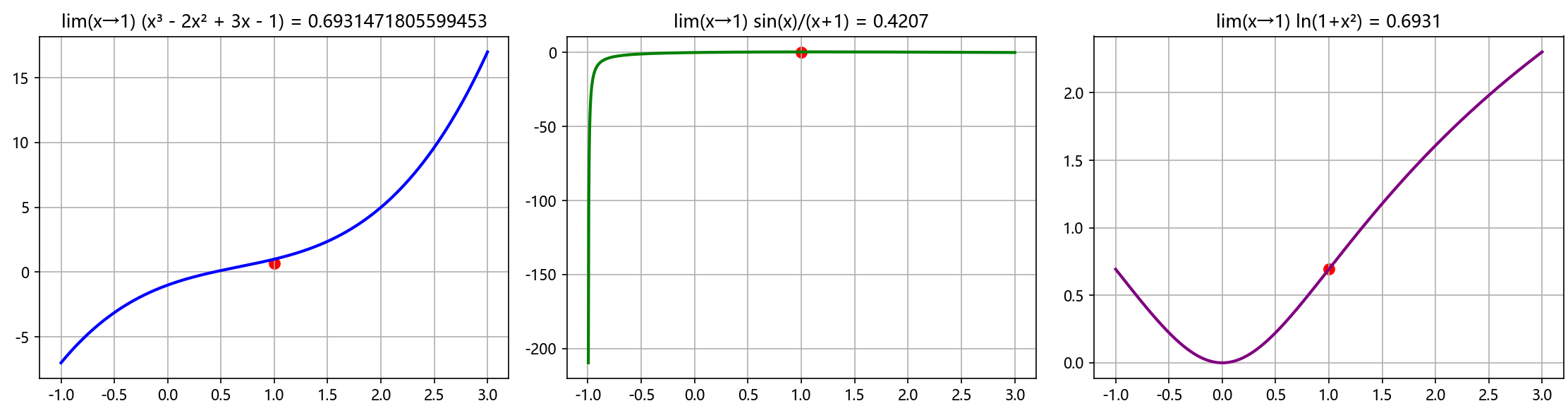
连续函数的性质在极限计算中有着重要应用。由于初等函数在其定义域内连续,我们可以直接代入计算极限值。
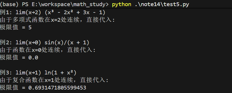
def demonstrate_continuity_in_limit_calculation():print("连续函数在极限计算中的应用示例:")print("=" * 50)# 示例1:多项式函数的极限def poly_func(x):return x**3 - 2*x**2 + 3*x - 1x0 = 2limit_value = poly_func(x0)print(f"例1: lim(x→{x0}) (x³ - 2x² + 3x - 1)")print(f"由于多项式函数在x={x0}处连续,直接代入:")print(f"极限值 = {limit_value}")print()# 示例2:三角函数的极限def trig_func(x):return np.sin(x) / (x + 1) # 在x=0处连续x0 = 0limit_value = trig_func(x0)print(f"例2: lim(x→{x0}) sin(x)/(x + 1)")print(f"由于函数在x={x0}处连续,直接代入:")print(f"极限值 = {limit_value}")print()# 示例3:复合函数的极限def composite_func(x):return np.log(1 + x**2) # 在x=1处连续x0 = 1limit_value = composite_func(x0)print(f"例3: lim(x→{x0}) ln(1 + x²)")print(f"由于复合函数在x={x0}处连续,直接代入:")print(f"极限值 = {limit_value}")print()# 可视化验证x = np.linspace(-1, 3, 1000)plt.figure(figsize=(15, 4))plt.subplot(1, 3, 1)y1 = poly_func(x)plt.plot(x, y1, 'b-', linewidth=2)plt.scatter([x0], [limit_value], color='red', s=50)plt.title(f'lim(x→{x0}) (x³ - 2x² + 3x - 1) = {limit_value}')plt.grid(True)plt.subplot(1, 3, 2)y2 = trig_func(x)plt.plot(x, y2, 'g-', linewidth=2)plt.scatter([x0], [trig_func(x0)], color='red', s=50)plt.title(f'lim(x→{x0}) sin(x)/(x+1) = {trig_func(x0):.4f}')plt.grid(True)plt.subplot(1, 3, 3)y3 = composite_func(x)plt.plot(x, y3, 'purple', linewidth=2)plt.scatter([x0], [composite_func(x0)], color='red', s=50)plt.title(f'lim(x→{x0}) ln(1+x²) = {composite_func(x0):.4f}')plt.grid(True)plt.tight_layout()plt.show()demonstrate_continuity_in_limit_calculation()
总结
通过本文的分析和Python可视化,我们可以清晰地看到:
- 连续函数的运算性质:连续函数经过四则运算和复合运算后,在满足条件的情况下仍然保持连续性
- 初等函数的连续性:所有初等函数在其定义域内都是连续的
- 实际应用价值:连续性性质大大简化了极限计算,对于连续函数可以直接代入求极限
这些性质不仅是数学分析的理论基础,也在工程计算和科学研究中有着广泛的应用。通过Python可视化,我们能够更直观地理解这些抽象的数学概念,将理论与实践完美结合。
关键词:连续函数、初等函数、极限计算、Python可视化、微积分
参考资料:
- 扈志明,《微积分》,高等教育出版社
欢迎点赞、收藏、评论,您的支持是我持续创作的最大动力!如有任何疑问,欢迎在评论区提出,我会尽快解答。。