当前位置：首页 > news >正文

快速上手大模型：机器学习5（逻辑回归及其代价函数）

news 2025/10/23 10:09:55

目录

1 逻辑回归

1.1 肿瘤分类示例

1.2 逻辑函数(Logistic function)

1.3 逻辑回归模型

1.4 代码表达

2 决策边界(Decision boundary)

2.1 定义

2.2 推导

3 逻辑回归的代价函数

3.1 数据集

3.2 代价函数构建

3.3 简化代价函数

4 梯度下降

1 逻辑回归

1.1 肿瘤分类示例

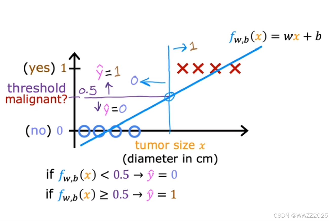
线性回归不适用这种分类，会改变肿瘤判断的标准，详情如下：

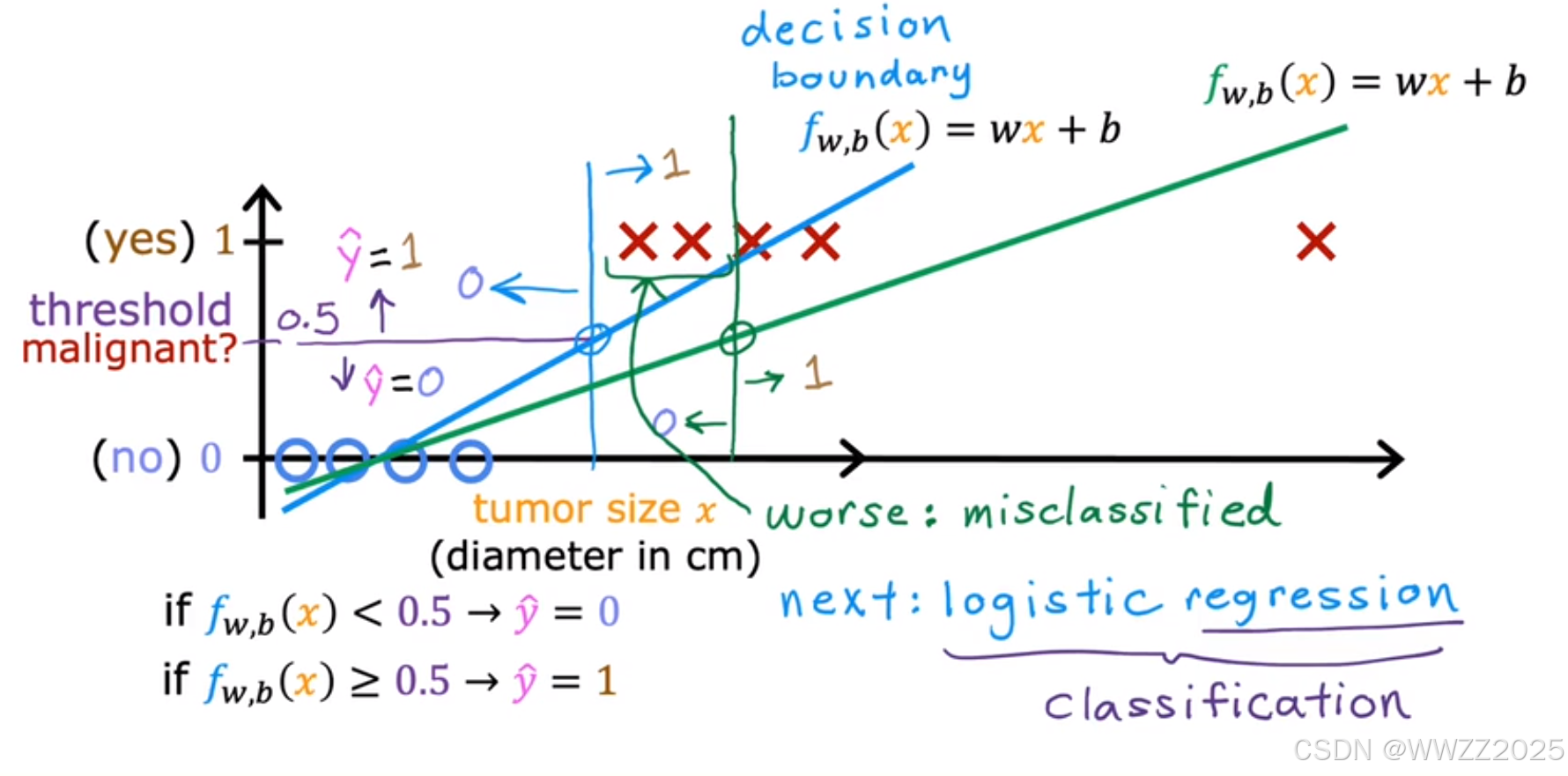
图中o为良性、x为恶性，是否为肿瘤阀值假设为0.5，则蓝色竖线（决策边界Decision boundary）左侧被判断为良性、右侧被判断为恶性；

当新增一个恶性肿瘤样本，线性回归最佳拟合曲线变成绿色的，阀值继续使用0.5时，样本中是恶性肿瘤的被判断为良性，原判断结论改变，预测有误。

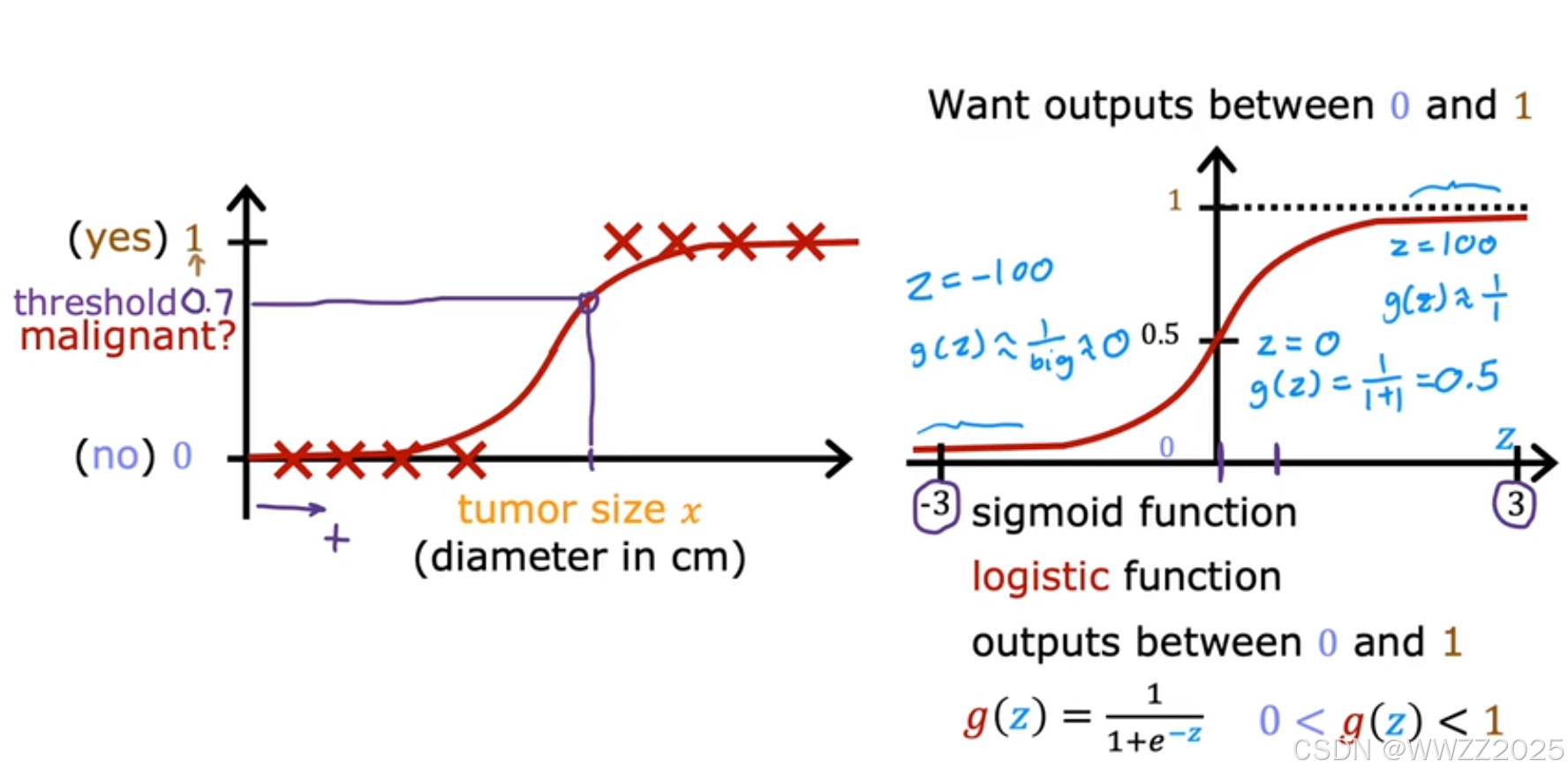
1.2 逻辑函数(Logistic function)

逻辑函数也称(sigmoid function)，定义式为 $g(z)=\frac{1}{1+e^{-z}},0<g(z)<1$ ，图像如下右图。

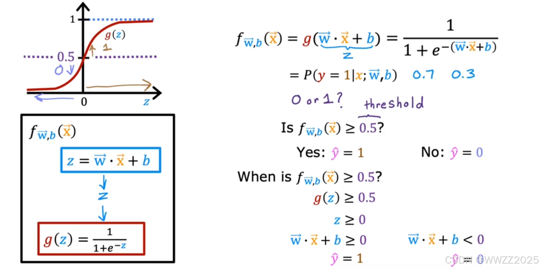
1.3 逻辑回归模型

模型： $z=\vec{w}*\vec{x}+b$

逻辑函数： $g(z)=\frac{1}{1+e^{-z}},0<g(z)<1$

逻辑回归模型： $f_{\vec{w},b}(\vec{x})=g(\vec{w}*\vec{x}+b)=\frac{1}{1+e^{-(\vec{w}*\vec{x}+b)}}$

肿瘤分类例子：

x：肿瘤大小

y：肿瘤良性/恶性的概率

如果 $f_{\vec{w},b}(\vec{x})=0.7$ ，则表示70%的概率肿瘤为恶性。

1.4 代码表达

import numpy as np
%matplotlib widget
import matplotlib.pyplot as plt
from plt_one_addpt_onclick import plt_one_addpt_onclick
from lab_utils_common import draw_vthresh
plt.style.use('./deeplearning.mplstyle')# Input is an array. 
input_array = np.array([1,2,3])
exp_array = np.exp(input_array)print("Input to exp:", input_array)
print("Output of exp:", exp_array)# Input is a single number
input_val = 1  
exp_val = np.exp(input_val)print("Input to exp:", input_val)
print("Output of exp:", exp_val)def sigmoid(z):"""Compute the sigmoid of zArgs:z (ndarray): A scalar, numpy array of any size.Returns:g (ndarray): sigmoid(z), with the same shape as z"""g = 1/(1+np.exp(-z))return g# Generate an array of evenly spaced values between -10 and 10
z_tmp = np.arange(-10,11)# Use the function implemented above to get the sigmoid values
y = sigmoid(z_tmp)# Code for pretty printing the two arrays next to each other
np.set_printoptions(precision=3) 
print("Input (z), Output (sigmoid(z))")
print(np.c_[z_tmp, y])

输出：

Input (z), Output (sigmoid(z))
[[-1.000e+01  4.540e-05][-9.000e+00  1.234e-04][-8.000e+00  3.354e-04][-7.000e+00  9.111e-04][-6.000e+00  2.473e-03][-5.000e+00  6.693e-03][-4.000e+00  1.799e-02][-3.000e+00  4.743e-02][-2.000e+00  1.192e-01][-1.000e+00  2.689e-01][ 0.000e+00  5.000e-01][ 1.000e+00  7.311e-01][ 2.000e+00  8.808e-01][ 3.000e+00  9.526e-01][ 4.000e+00  9.820e-01][ 5.000e+00  9.933e-01][ 6.000e+00  9.975e-01][ 7.000e+00  9.991e-01][ 8.000e+00  9.997e-01][ 9.000e+00  9.999e-01][ 1.000e+01  1.000e+00]]

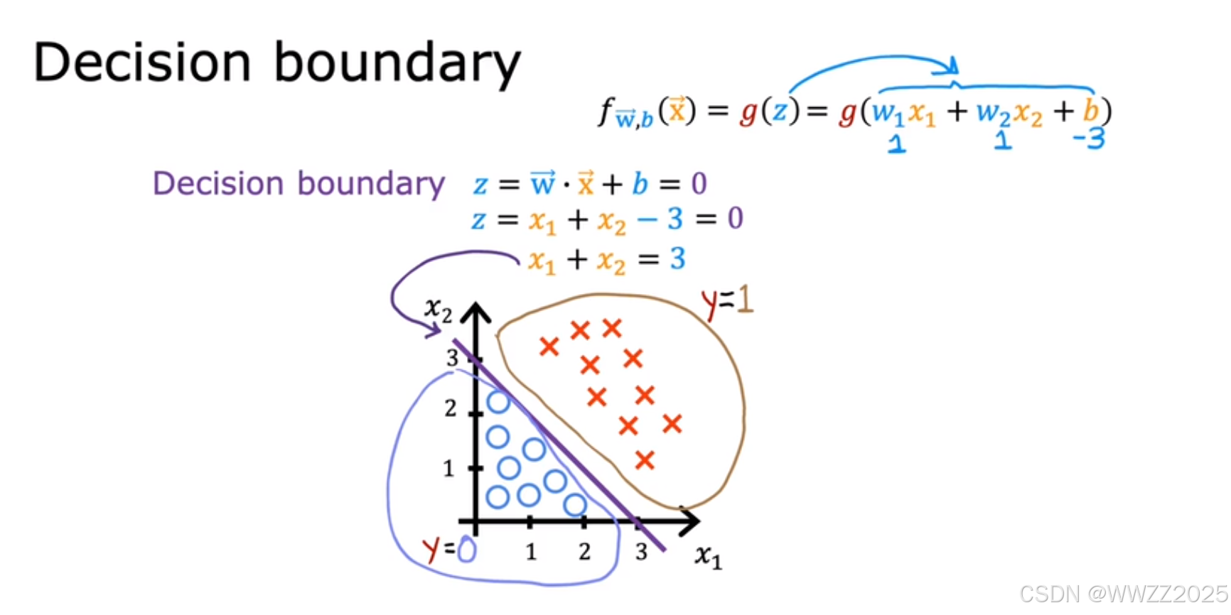
2 决策边界(Decision boundary)

2.1 定义

用于决策判断的分割线。

2.2 推导

当逻辑回归模型为 $f_{\vec{w},b}(\vec{x})=g(\vec{w}*\vec{x}+b)=\frac{1}{1+e^{-(\vec{w}*\vec{x}+b)}}$ ，

如果 $f\geqslant 0.5$ ，则 $g\geqslant 0.5$ 、 $z\geqslant 0$ 、 $\vec{w}*\vec{x}+b\geqslant 0$ ，输出 $\hat{y}=1$ ，此时预测为恶性。

另w1=w2=1,b=-3

则决策边界为 $z= 0$ ，即 $x_{1}+x_{2}=3$

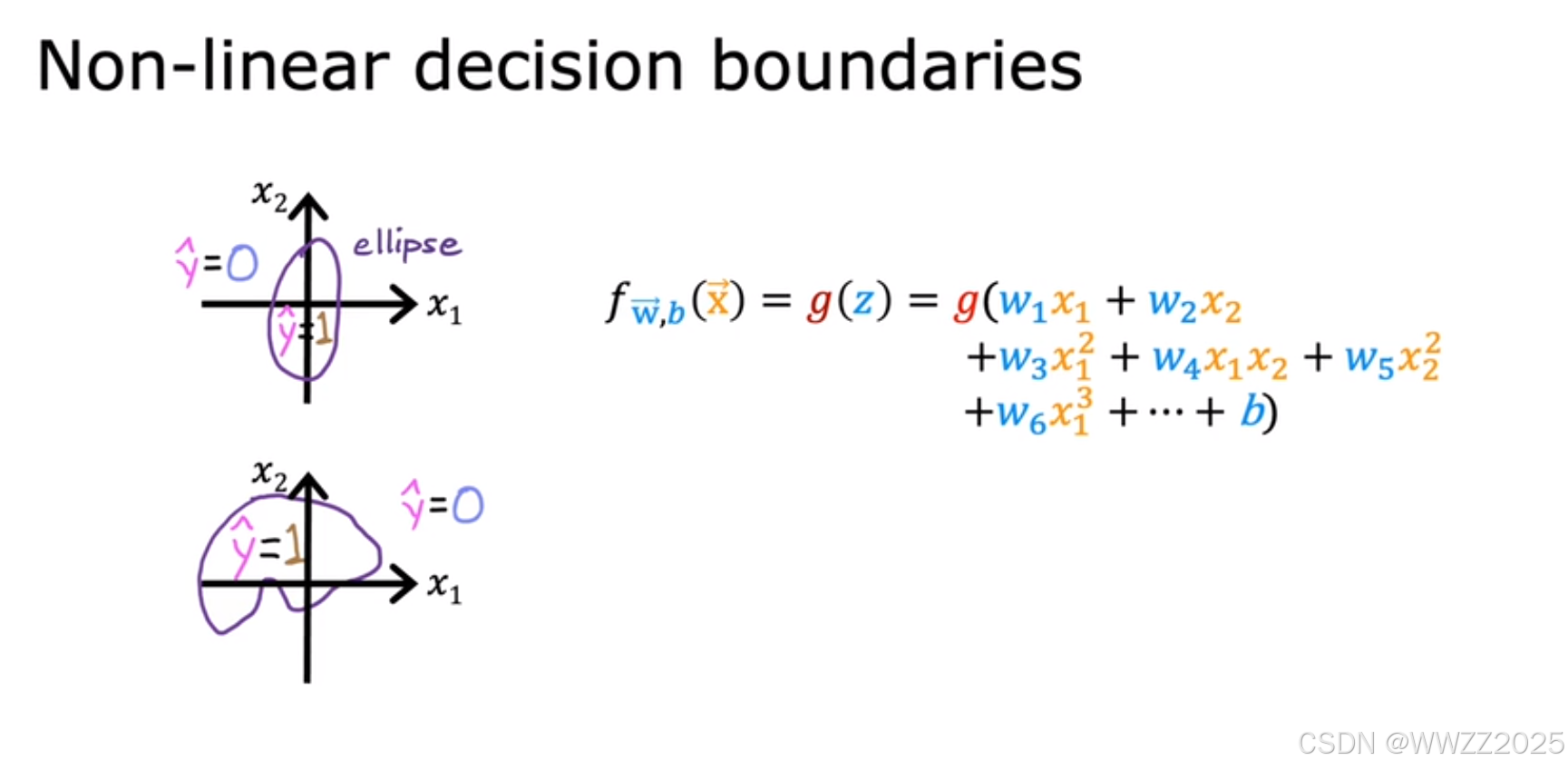
非线性决策边界同理。

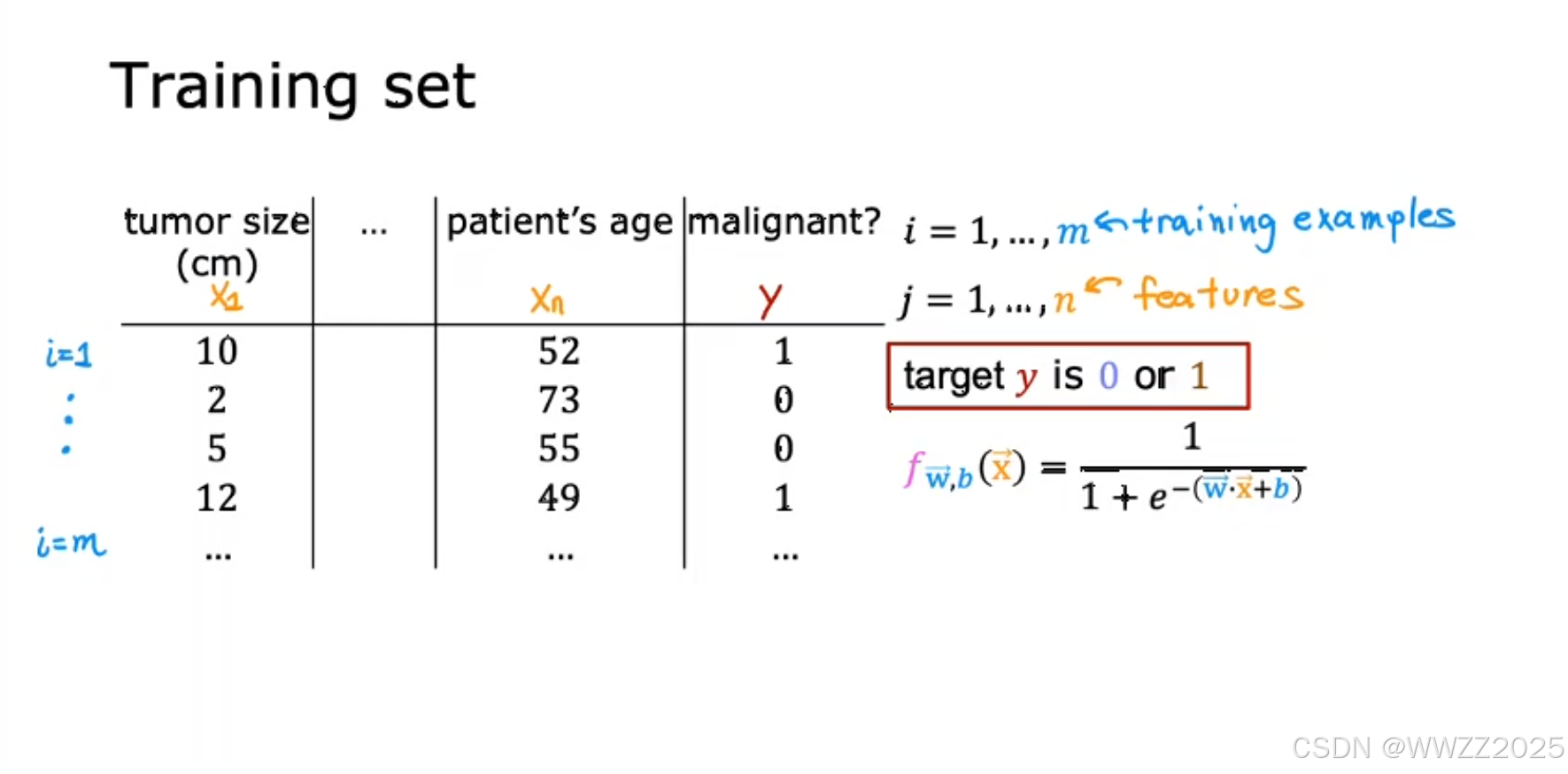
3 逻辑回归的代价函数

3.1 数据集

m为训练样本数量，m为特征，y为目标标签，逻辑回归模型为 $f_{\vec{w},b}(\vec{x})=\frac{1}{1+e^{-(\vec{w}*\vec{x}+b)}}$

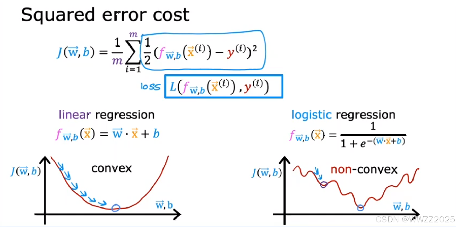
3.2 代价函数构建

逻辑回归的代价函数不用平方差误差函数，会出现如上右图所示非凸代价函数(non-convex)，即多个局部最小值情况。

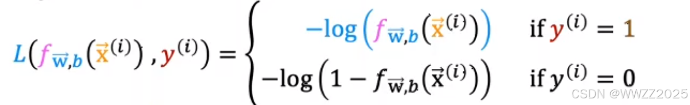
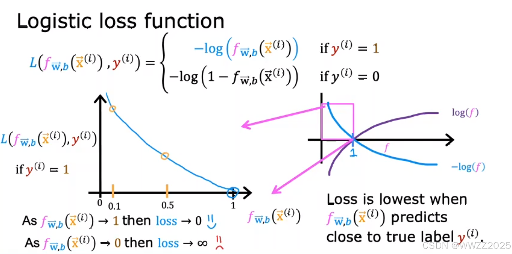
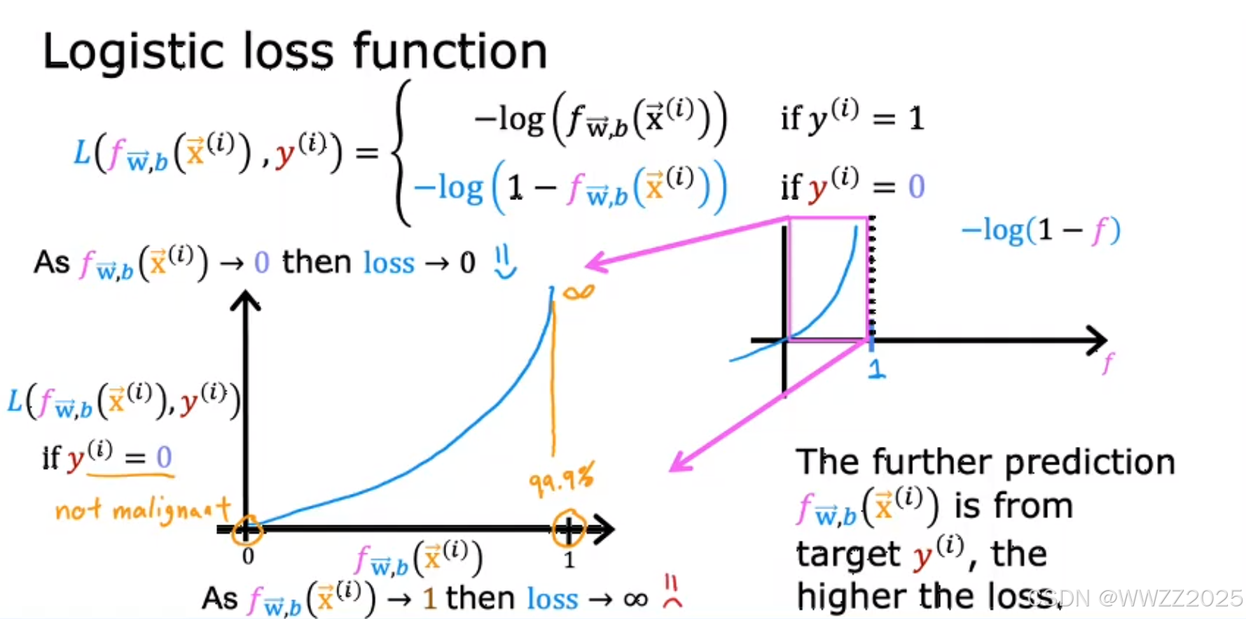
因此，另损失 $L=(f_{\vec{w,b}}(\vec{x}^{(i)}),y^{(i)})$ ，函数式如下：

当真实值为1，预测值越接近1，损失L就越小；

当真实值为0，预测值越接近0，损失L就越小。

3.3 简化代价函数

损失： $L(f_{\vec{w,b}}(\vec{x}^{(i)}),y^{(i)})=-y^{(i)}log(f_{\vec{w,b}}(\vec{x}^{(i)})-(1-y^{(i)})log(1-f_{\vec{w,b}}(\vec{x}^{(i)})$

代价函数： $J(\vec{w},b)=\frac{1}{m}\sum_{i=1}^{m}L(f_{\vec{w,b}}(\vec{x}^{(i)}),y^{(i)})$

$-\frac{1}{m}\sum_{i=1}^{m}[y^{(i)}log(f_{\vec{w,b}}(\vec{x}^{(i)})+(1-y^{(i)})log(1-f_{\vec{w,b}}(\vec{x}^{(i)})]$

4 梯度下降

代价函数： $J(\vec{w},b)=-\frac{1}{m}\sum_{i=1}^{m}[y^{(i)}log(f_{\vec{w,b}}(\vec{x}^{(i)})+(1-y^{(i)})log(1-f_{\vec{w,b}}(\vec{x}^{(i)})]$

梯度下降： $w_{j}=w_{j}-\alpha \frac{\partial J(\vec{w},b)}{\partial w_{j}}=\frac{1}{m}\sum_{i=1}^{m}(f_{\vec{w,b}}(\vec{x}^{(i)}),y^{(i)})\vec{x}_{j}^{(i)}$

$b=b-\alpha \frac{\partial J(\vec{w},b)}{\partial b}=\frac{1}{m}\sum_{i=1}^{m}(f_{\vec{w,b}}(\vec{x}^{(i)}),y^{(i)})$