python物理模拟：描述波动、振动和旋转系统

目录

概述

1 理论背景

2 物理模拟设计

2.1 简谐振动

2.1.1 理论介绍

2.1.2  简谐振动模拟

2.2 波动传播模拟

2.2.1 理论介绍

2.2.2 波动传播模拟

2.3 二维水波模拟

2.3.1 理论介绍

2.3.2  简谐振动模拟

2.4 耦合振子模拟

2.3.1 理论介绍

2.3.2  耦合振子模拟

2.5 傅科摆模拟 - 地球自转效应

2.5.1 理论介绍

2.5.2  傅科摆模拟 - 地球自转效应

2.6 量子力学波包演化模拟

2.6.1 理论介绍

2.6.2  量子力学波包演化模拟

2.7 电磁波传播模拟

2.7.1 理论介绍

2.7.2 电磁波传播模拟

---

概述

本文主要介绍使用python工具模拟一下常见的物理模型，其可通过将数学公式通过python语言表述出来，并通过图像呈现出来，这些模型主要包括：描述波动、振动和旋转系统。

1 理论背景

欧拉公式在物理模拟中非常有用，特别是在描述波动、振动和旋转系统时。我们可以利用欧拉公式将三角函数用复指数表示，从而简化计算。以下是一些物理模拟的例子：

1. 简谐振动：可以使用复数形式表示振动，然后取实部或虚部得到实际的物理量。

2. 波动方程：一维或二维波动可以用复数形式表示，便于处理波的叠加和传播。

3. 旋转系统：例如刚体的旋转，可以用复数表示旋转操作。

笔者用Python模拟以下场景：

• 简谐振动的位移、速度和加速度。

• 两个简谐振动叠加形成的拍频。

• 二维波动传播（例如水波）。

• 旋转的矢量（例如表示一个在复平面上旋转的复数）。

2 物理模拟设计

2.1 简谐振动

2.1.1 理论介绍

简谐振动是物理学和工程学中最基本和重要的振动形式。它描述了一个系统在恢复力与位移成正比且方向相反的条件下的运动。下面详细解释简谐振动理论，包括其数学描述、特征和能量分析。

简谐振动的运动方程由胡克定律给出：

    F=−kx

其中，F 是恢复力，k 是劲度系数，x 是位移。

简谐振动的定义

简谐振动是指一个系统在恢复力与位移成正比且方向相反的作用下进行的振动。其基本特征：

• 恢复力：F = -kx

• 运动方程：m(d²x/dt²) = -kx

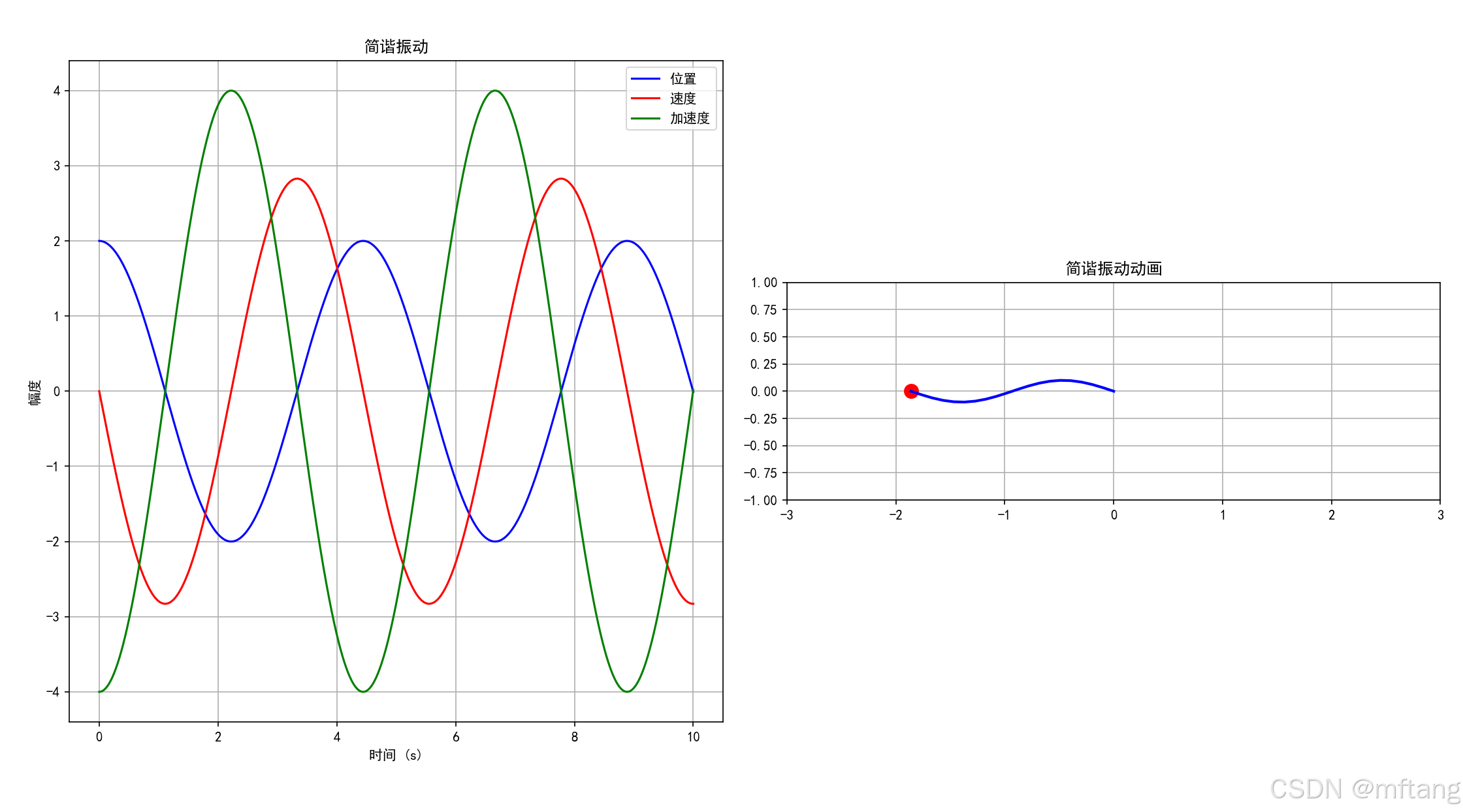
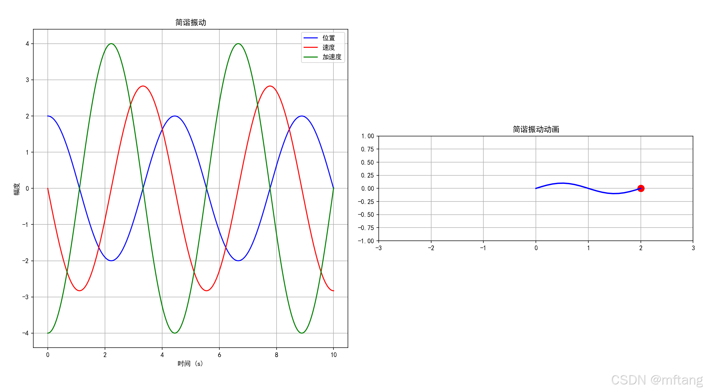
2.1.2  简谐振动模拟

1) 源代码

import numpy as np
import matplotlib.pyplot as plt
from matplotlib.animation import FuncAnimationclass HarmonicOscillator:"""简谐振动模拟器"""def __init__(self, mass=1.0, k=1.0, amplitude=1.0, phase=0):self.mass = massself.k = k  # 弹簧常数self.amplitude = amplitudeself.phase = phaseself.omega = np.sqrt(k / mass)  # 角频率def position(self, t):"""使用欧拉公式计算位置"""return self.amplitude * np.real(np.exp(1j * (self.omega * t + self.phase)))def velocity(self, t):"""使用欧拉公式计算速度"""return self.amplitude * self.omega * np.real(1j * np.exp(1j * (self.omega * t + self.phase)))def acceleration(self, t):"""使用欧拉公式计算加速度"""return -self.amplitude * self.omega**2 * np.real(np.exp(1j * (self.omega * t + self.phase)))def animate_harmonic_oscillator():"""简谐振动动画"""oscillator = HarmonicOscillator(mass=1.0, k=2.0, amplitude=2.0)fig, (ax1, ax2) = plt.subplots(1, 2, figsize=(12, 5))# 时间数组t_max = 10t = np.linspace(0, t_max, 1000)# 计算位置、速度和加速度x = [oscillator.position(ti) for ti in t]v = [oscillator.velocity(ti) for ti in t]a = [oscillator.acceleration(ti) for ti in t]# 绘制静态曲线ax1.plot(t, x, 'b-', label='位置')ax1.plot(t, v, 'r-', label='速度')ax1.plot(t, a, 'g-', label='加速度')ax1.set_xlabel('时间 (s)')ax1.set_ylabel('幅度')ax1.set_title('简谐振动')ax1.legend()ax1.grid(True)# 动画部分mass_point, = ax2.plot([], [], 'ro', markersize=10)spring, = ax2.plot([], [], 'b-', linewidth=2)ax2.set_xlim(-3, 3)ax2.set_ylim(-1, 1)ax2.set_aspect('equal')ax2.set_title('简谐振动动画')ax2.grid(True)def init():mass_point.set_data([], [])spring.set_data([], [])return mass_point, springdef animate(frame):current_time = frame * t_max / 100current_x = oscillator.position(current_time)# 更新质量块位置mass_point.set_data([current_x], [0])# 更新弹簧spring_x = np.linspace(0, current_x, 20)spring_y = 0.1 * np.sin(spring_x * 2 * np.pi / (current_x if current_x != 0 else 1))spring.set_data(spring_x, spring_y)return mass_point, springani = FuncAnimation(fig, animate, frames=100, init_func=init, blit=True, interval=50)plt.tight_layout()plt.show()animate_harmonic_oscillator()

2） 运行结果

2.2 波动传播模拟

2.2.1 理论介绍

波动传播理论是物理学和工程学中的一个核心课题，涉及波在介质中传播的规律。波可以分为机械波（如声波、水波）、电磁波（如光波、无线电波）等。波动传播理论通常包括波动的描述、波动方程、波的叠加、干涉、衍射、驻波、多普勒效应等内容。

一维波动方程描述了波在一条直线上的传播：

∂²u/∂t² = c² ∂²u/∂x²

其中：

• u(x,t) 是波函数

• c 是波速

• x 是位置

• t 是时间

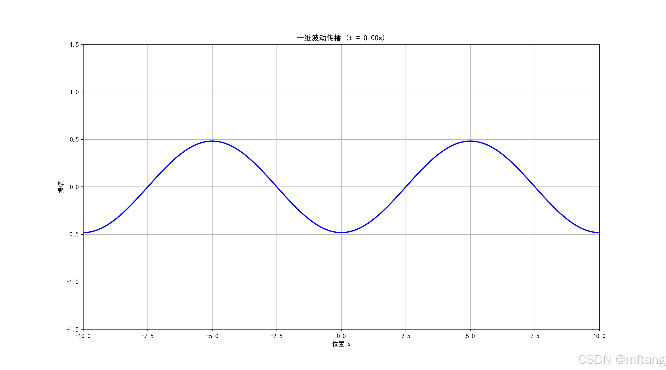
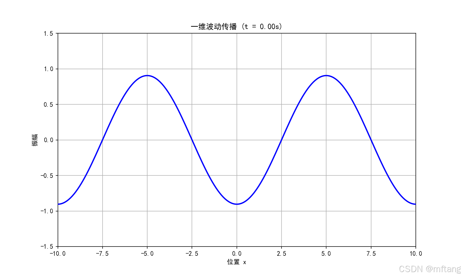
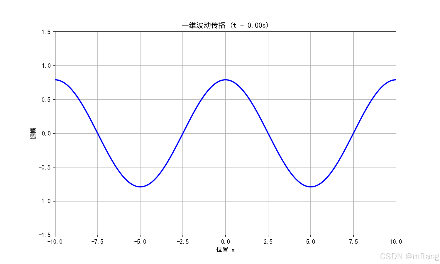
2.2.2 波动传播模拟

1） 代码实现

def wave_propagation_simulation():"""一维波动传播模拟"""# 参数设置L = 10.0  # 空间范围T = 5.0   # 时间范围c = 1.0   # 波速# 网格x = np.linspace(-L, L, 200)t = np.linspace(0, T, 100)# 创建波函数 - 使用复数表示k = 2 * np.pi / L  # 波数omega = c * k      # 角频率# 初始化图形fig, ax = plt.subplots(figsize=(10, 6))line, = ax.plot(x, np.zeros_like(x), 'b-', linewidth=2)ax.set_xlim(-L, L)ax.set_ylim(-1.5, 1.5)ax.set_xlabel('位置 x')ax.set_ylabel('振幅')ax.set_title('一维波动传播')ax.grid(True)def wave_function(x, t):"""使用复数表示的波动方程解"""# 向右传播的波wave_right = np.real(np.exp(1j * (k * x - omega * t)))# 向左传播的波wave_left = np.real(np.exp(1j * (k * x + omega * t)))# 叠加return 0.5 * (wave_right + wave_left)def animate(frame):current_time = frame * T / len(t)y = wave_function(x, current_time)line.set_ydata(y)ax.set_title(f'一维波动传播 (t = {current_time:.2f}s)')return line,ani = FuncAnimation(fig, animate, frames=len(t), interval=50, blit=True)plt.show()wave_propagation_simulation()

2)  运行结果

2.3 二维水波模拟

2.3.1 理论介绍

二维水波理论主要研究液体表面波的传播，通常基于势流理论，假设流体无粘、不可压缩且流动无旋。对于二维水波，考虑在x方向传播，在z方向有自由表面的波。控制方程是拉普拉斯方程，边界条件包括自由表面的动力和运动边界条件。

将模拟二维水波，考虑重力作用，忽略表面张力。采用简单的数值方法：在规则网格上求解拉普拉斯方程，然后更新自由表面的边界条件。

然而，直接求解拉普拉斯方程和自由表面边界条件较为复杂。这里采用一种简化的方法：使用线性波理论（Airy波）的解析解，以及一种常见的数值方法——使用Height Field（高度场）和快速傅里叶变换（FFT）的方法。

另一种常见的方法是使用浅水方程或Boussinesq方程，但这里使用基于FFT的方法，该方法适用于深水波。

基于FFT的方法（如Tessendorf方法）常用于模拟海洋表面，它通过叠加不同频率和方向的正弦波来生成水波。我们将实现一个简单的版本。

二维水波理论基于以下假设：

• 流体无粘、不可压缩

• 流动无旋（存在速度势）

• 波幅相对于波长较小

• 底部水平

控制方程：

• 拉普拉斯方程：∇²φ = 0 （在流体内部）

• 自由表面动力学边界条件

• 自由表面运动学边界条件

• 底部边界条件

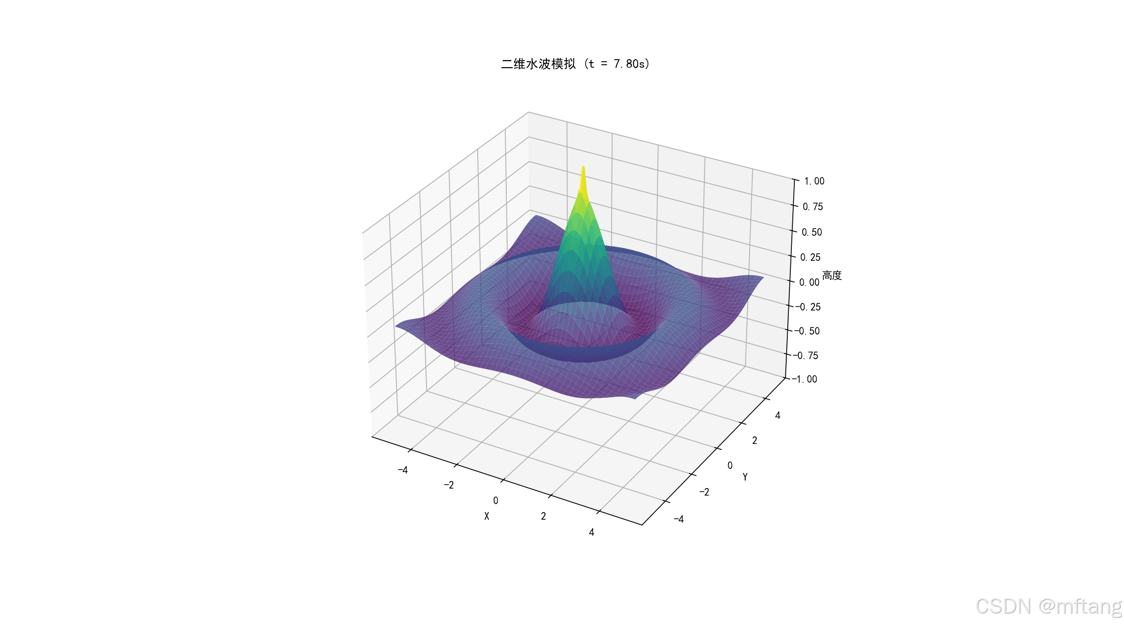
2.3.2  简谐振动模拟

1） 代码实现

def water_wave_simulation():"""二维水波模拟"""# 创建网格x = np.linspace(-5, 5, 100)y = np.linspace(-5, 5, 100)X, Y = np.meshgrid(x, y)# 参数k = 2.0  # 波数omega = 1.0  # 角频率A = 0.5  # 振幅fig = plt.figure(figsize=(10, 8))ax = fig.add_subplot(111, projection='3d')def wave_height(x, y, t):"""使用复数表示的水波高度"""r = np.sqrt(x**2 + y**2)# 避免除以零r = np.where(r == 0, 1e-10, r)# 使用复数表示的圆形波return A * np.real(np.exp(1j * (k * r - omega * t))) / rdef animate(frame):ax.clear()current_time = frame * 0.1Z = wave_height(X, Y, current_time)# 绘制表面surf = ax.plot_surface(X, Y, Z, cmap='viridis', alpha=0.8)ax.set_zlim(-1, 1)ax.set_title(f'二维水波模拟 (t = {current_time:.2f}s)')ax.set_xlabel('X')ax.set_ylabel('Y')ax.set_zlabel('高度')return surf,ani = FuncAnimation(fig, animate, frames=100, interval=50, blit=False)plt.show()water_wave_simulation()

2） 运行结果

2.4 耦合振子模拟

2.3.1 理论介绍

从最简单的两个耦合振子开始，然后推广到多个振子，并分析其简正模。将使用数值模拟和解析分析相结合的方法。

1. 两个耦合振子的运动方程
   考虑两个相同质量的振子，每个振子与固定端通过弹簧常数k连接，两个振子之间通过弹簧常数k_c连接。设两个振子的位移分别为x1和x2，则运动方程为：

   m * d²x1/dt² = -k * x1 - k_c * (x1 - x2)
   m * d²x2/dt² = -k * x2 - k_c * (x2 - x1)

2. 简正模分析
   通过引入简正坐标，可以将耦合振子系统解耦为独立的简正模。对于两个振子，简正模为对称模和反对称模。

3. 多个耦合振子
   我们将考虑一维链上的多个耦合振子，并分析其简正模和色散关系。

4. 同步现象
   耦合振子中一个有趣的现象是同步，即振子之间通过耦合调整频率和相位，最终达到相同的振荡频率或固定的相位关系。

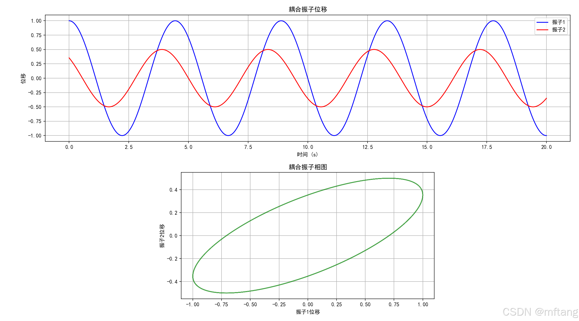
2.3.2  耦合振子模拟

1） 代码实现

def coupled_oscillators():"""耦合振子模拟"""# 参数m1, m2 = 1.0, 1.0  # 质量k1, k2, k3 = 1.0, 1.0, 1.0  # 弹簧常数# 计算简正模频率omega1 = np.sqrt((k1 + k2) / m1)omega2 = np.sqrt((k2 + k3) / m2)# 初始条件A1, A2 = 1.0, 0.5  # 振幅phi1, phi2 = 0, np.pi / 4  # 相位# 时间数组t = np.linspace(0, 20, 1000)# 计算位移x1 = A1 * np.cos(omega1 * t + phi1)x2 = A2 * np.cos(omega2 * t + phi2)# 绘制结果fig, (ax1, ax2) = plt.subplots(2, 1, figsize=(10, 8))ax1.plot(t, x1, 'b-', label='振子1')ax1.plot(t, x2, 'r-', label='振子2')ax1.set_xlabel('时间 (s)')ax1.set_ylabel('位移')ax1.set_title('耦合振子位移')ax1.legend()ax1.grid(True)# 相图ax2.plot(x1, x2, 'g-', alpha=0.7)ax2.set_xlabel('振子1位移')ax2.set_ylabel('振子2位移')ax2.set_title('耦合振子相图')ax2.grid(True)ax2.set_aspect('equal')plt.tight_layout()plt.show()

2） 运行结果

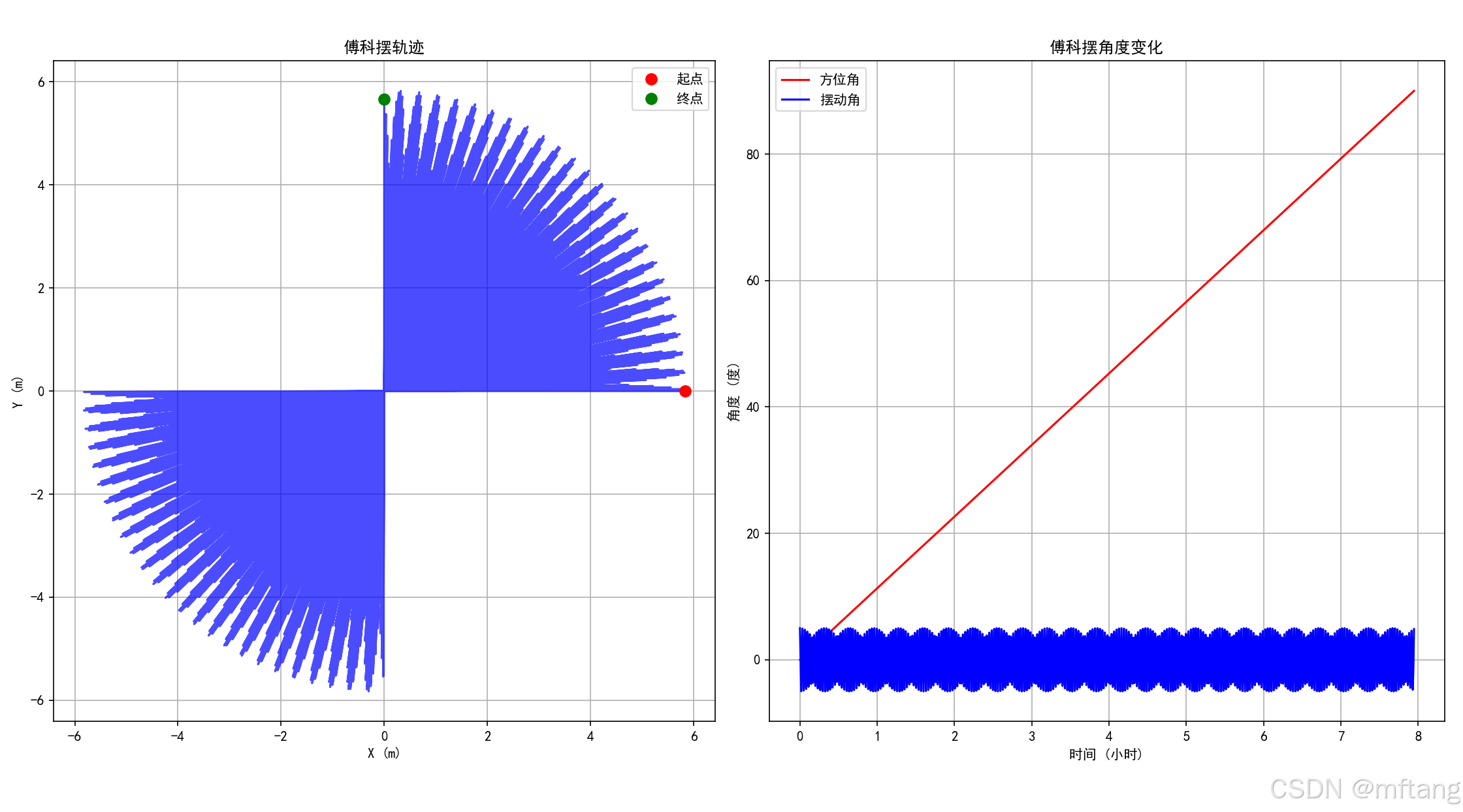
2.5 傅科摆模拟 - 地球自转效应

2.5.1 理论介绍

2.5.2  傅科摆模拟 - 地球自转效应

1） 代码实现

def foucault_pendulum_simulation():"""傅科摆模拟 - 地球自转效应"""# 参数latitude = np.radians(48.8566)  # 巴黎纬度 (度转弧度)omega_earth = 7.292e-5  # 地球自转角速度 (rad/s)pendulum_length = 67  # 摆长 (m)g = 9.81  # 重力加速度# 计算傅科摆的进动角速度omega_precession = omega_earth * np.sin(latitude)T_precession = 2 * np.pi / omega_precession  # 进动周期# 摆的运动周期T_pendulum = 2 * np.pi * np.sqrt(pendulum_length / g)print(f"傅科摆进动周期: {T_precession / 3600:.2f} 小时")print(f"摆的摆动周期: {T_pendulum:.2f} 秒")# 模拟t = np.linspace(0, T_precession / 4, 1000)  # 模拟1/4进动周期# 初始条件 - 摆从正北方向释放theta_0 = np.radians(5)  # 初始角度 (5度)# 摆的摆动 (不考虑阻尼)theta = theta_0 * np.cos(2 * np.pi / T_pendulum * t)# 由于地球自转引起的方位角变化phi = omega_precession * t# 转换为直角坐标x = pendulum_length * np.sin(theta) * np.cos(phi)y = pendulum_length * np.sin(theta) * np.sin(phi)# 绘制结果fig, (ax1, ax2) = plt.subplots(1, 2, figsize=(12, 5))# 轨迹图ax1.plot(x, y, 'b-', alpha=0.7)ax1.plot(x[0], y[0], 'ro', markersize=8, label='起点')ax1.plot(x[-1], y[-1], 'go', markersize=8, label='终点')ax1.set_xlabel('X (m)')ax1.set_ylabel('Y (m)')ax1.set_title('傅科摆轨迹')ax1.legend()ax1.grid(True)ax1.set_aspect('equal')# 角度随时间变化ax2.plot(t / 3600, np.degrees(phi), 'r-', label='方位角')ax2.plot(t / 3600, np.degrees(theta), 'b-', label='摆动角')ax2.set_xlabel('时间 (小时)')ax2.set_ylabel('角度 (度)')ax2.set_title('傅科摆角度变化')ax2.legend()ax2.grid(True)plt.tight_layout()plt.show()

2） 运行结果

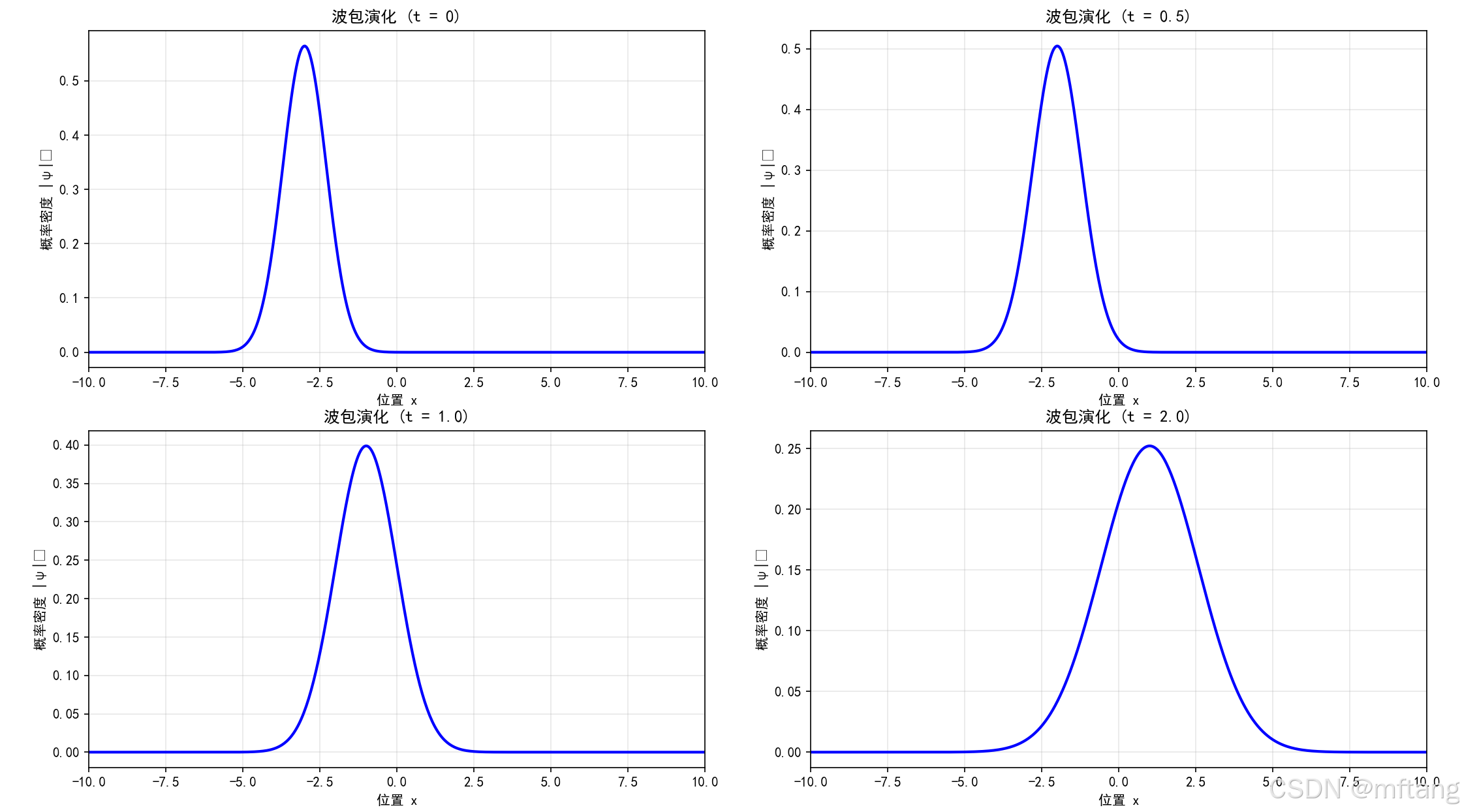
2.6 量子力学波包演化模拟

2.6.1 理论介绍

2.6.2  量子力学波包演化模拟

1） 代码实现

def quantum_wave_packet():"""量子力学波包演化模拟"""# 参数hbar = 1.0  # 简化普朗克常数m = 1.0  # 粒子质量# 空间网格x = np.linspace(-10, 10, 500)# 初始波包参数x0 = -3.0  # 初始位置k0 = 2.0  # 初始动量sigma = 1.0  # 波包宽度# 初始波函数 (高斯波包)psi_0 = (1 / (np.pi * sigma ** 2) ** 0.25) * np.exp(1j * k0 * x) * np.exp(-(x - x0) ** 2 / (2 * sigma ** 2))# 在动量空间中演化k = np.fft.fftfreq(len(x), x[1] - x[0]) * 2 * np.pipsi_k = np.fft.fft(psi_0)# 时间演化t_values = [0, 0.5, 1.0, 2.0]fig, axes = plt.subplots(2, 2, figsize=(12, 10))axes = axes.flatten()for i, t in enumerate(t_values):# 在动量空间中时间演化psi_k_t = psi_k * np.exp(-1j * hbar * k ** 2 * t / (2 * m))# 变换回坐标空间psi_t = np.fft.ifft(psi_k_t)# 绘制概率密度axes[i].plot(x, np.abs(psi_t) ** 2, 'b-', linewidth=2)axes[i].set_xlabel('位置 x')axes[i].set_ylabel('概率密度 |ψ|²')axes[i].set_title(f'波包演化 (t = {t})')axes[i].grid(True, alpha=0.3)axes[i].set_xlim(-10, 10)plt.tight_layout()plt.show()

2） 运行结果

2.7 电磁波传播模拟

2.7.1 理论介绍

麦克斯韦方程组是电磁理论的基础：

• ∇·E = ρ/ε₀

• ∇·B = 0

• ∇×E = -∂B/∂t

• ∇×B = μ₀J + μ₀ε₀∂E/∂t

在真空中（ρ=0, J=0），可以得到波动方程：

• ∇²E - (1/c²)∂²E/∂t² = 0

• ∇²B - (1/c²)∂²B/∂t² = 0

其中 c = 1/√(μ₀ε₀) 是光速

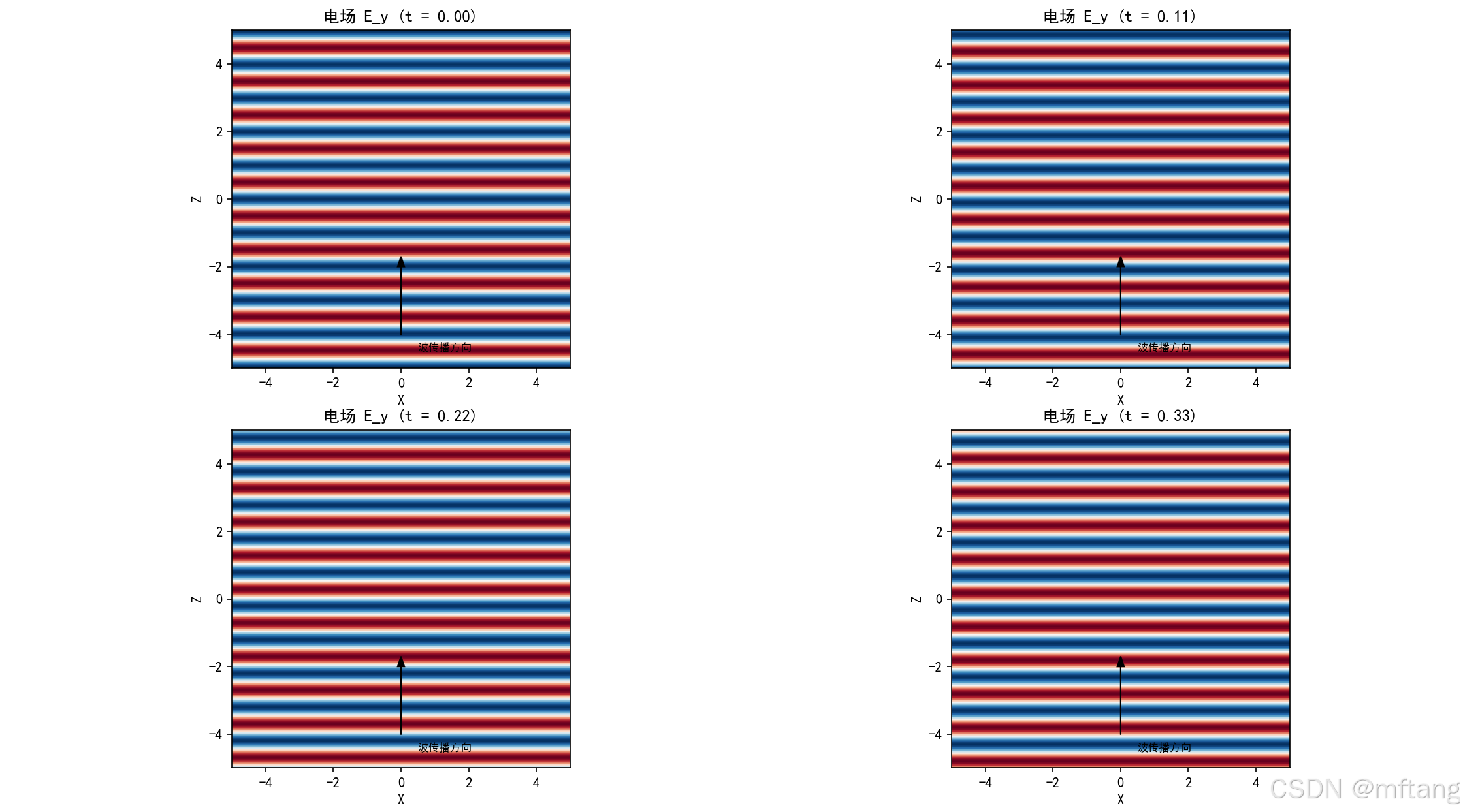
2.7.2 电磁波传播模拟

1） 代码实现

import matplotlib
import numpy as np
import matplotlib.pyplot as pltmatplotlib.use('TkAgg')# 设置支持中文的字体
plt.rcParams['font.sans-serif'] = ['SimHei']  # 用来正常显示中文标签（黑体）
plt.rcParams['axes.unicode_minus'] = False  # 用来正常显示负号import numpy as np
import matplotlib.pyplot as plt
from matplotlib.animation import FuncAnimationdef electromagnetic_wave_simulation():"""电磁波传播模拟"""# 参数c = 1.0  # 光速wavelength = 1.0k = 2 * np.pi / wavelength  # 波数omega = c * k  # 角频率# 空间网格x = np.linspace(-5, 5, 200)z = np.linspace(-5, 5, 200)X, Z = np.meshgrid(x, z)# 时间t = np.linspace(0, 2 * np.pi / omega, 10)fig, axes = plt.subplots(2, 2, figsize=(10, 10))for i, time in enumerate(t[:4]):# 电场 (沿y方向极化)E_y = np.real(np.exp(1j * (k * Z - omega * time)))# 磁场 (沿x方向)B_x = np.real(np.exp(1j * (k * Z - omega * time))) / cax = axes[i // 2, i % 2]im = ax.imshow(E_y, extent=(-5, 5, -5, 5), cmap='RdBu', vmin=-1, vmax=1)ax.set_title(f'电场 E_y (t = {time:.2f})')ax.set_xlabel('X')ax.set_ylabel('Z')# 添加波传播方向ax.arrow(0, -4, 0, 2, head_width=0.2, head_length=0.3, fc='k', ec='k')ax.text(0.5, -4.5, '波传播方向', fontsize=8)plt.tight_layout()plt.show()

2） 运行结果