当前位置：首页 > news >正文

「机器学习笔记14」集成学习全面解析：从Bagging到Boosting的Python实战指南

news 2025/10/15 9:25:04

三个臭皮匠，顶个诸葛亮。在机器学习领域，集成学习正是这一智慧的最佳体现。

一、什么是集成学习？

集成学习（Ensemble Learning）是一种通过构建并结合多个学习器来完成学习任务的机器学习方法。其核心思想是：将多个弱学习器组合起来，形成一个强学习器，从而获得比单一学习器更优越的性能。

1.1 集成学习的理论基础

为什么集成学习有效？主要有四个关键原因：

1. 经验法则的局限性

很容易找到非常正确的"经验法则"，但很难找到单个高准确率的规则
多个近似正确的规则组合起来可能达到更好的效果

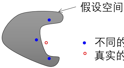
2. 假设空间的多解性 当训练样本很少而假设空间很大时，可能存在多个同样精度的假设。选择某一个假设可能在测试集上效果较差，而集成多个假设可以降低风险。

3. 避免局部最优 算法可能会收敛到局部最优解。融合不同的假设可以降低收敛到不好局部最优的风险。

4. 假设空间的局限性 真实假设可能不在当前算法定义的假设空间中，但多个近似假设的组合可能更好地逼近真实假设。

1.2 强学习器 vs 弱学习器

强学习器：有高准确度的学习算法
弱学习器：在任何训练集上可以做到比随机预测略好（错误率 $error=1/2−γ\text{error} = 1/2 - \gamma$ ）

集成学习的关键问题：我们能否把一个弱学习器增强成一个强学习器？

二、集成学习的主要方法

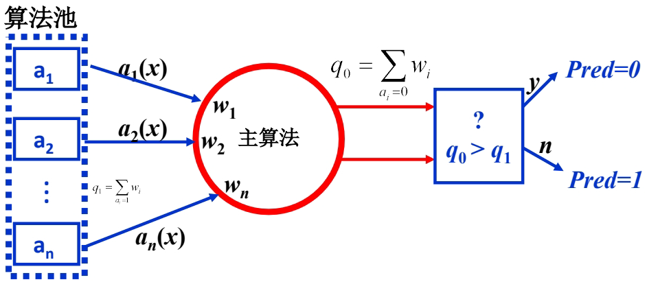
2.1 加权多数算法（Weighted Majority Algorithm）

加权多数算法是最早的集成学习方法之一，适用于二分类问题。

算法原理

预测阶段：

每个算法 $a_i$ 对输入 $x$ 产生二值输出 ${0,1\}$
计算加权投票： $q0=∑ai=0wiq_0 = \sum_{a_i=0} w_i$ ， $q1=∑ai=1wiq_1 = \sum_{a_i=1} w_i$
最终预测：如果 $q_0 > q_1$ 则预测为0，否则预测为1

训练阶段：

初始化所有权重 $w_i = 1$
对每个训练样本 $⟨x,c(x)⟩\langle x, c(x) \rangle$ ：
- 计算加权投票并作出预测
- 对预测错误的算法： $wi←βwiw_i \leftarrow \beta w_i$ （ $β∈[0](@ref)[1](@ref)\beta \in [0](@ref)[1](@ref)$ 是惩罚系数）

Python实现示例

import numpy as np
from sklearn.base import BaseEstimator, ClassifierMixinclass WeightedMajorityClassifier(BaseEstimator, ClassifierMixin):def __init__(self, base_estimators, beta=0.5):self.base_estimators = base_estimatorsself.beta = betaself.weights = Nonedef fit(self, X, y):n_estimators = len(self.base_estimators)self.weights = np.ones(n_estimators)# 训练所有基学习器for estimator in self.base_estimators:estimator.fit(X, y)return selfdef predict(self, X):predictions = np.array([estimator.predict(X) for estimator in self.base_estimators])weighted_votes = np.dot(self.weights, predictions)return np.where(weighted_votes >= 0, 1, 0)def partial_fit(self, X, y):"""在线学习：根据新数据更新权重"""if self.weights is None:self.weights = np.ones(len(self.base_estimators))# 获取当前预测current_predictions = self.predict(X)# 更新权重for i, estimator in enumerate(self.base_estimators):estimator_prediction = estimator.predict(X)if estimator_prediction != y:self.weights[i] *= self.beta# 归一化权重self.weights /= np.sum(self.weights)return self

2.2 Bagging（Bootstrap Aggregating）

Bagging通过自助采样法构建多个训练集，分别训练基学习器，然后通过投票或平均法结合预测结果。

Bootstrap采样原理

从包含m个样本的数据集D中，有放回地随机抽取m个样本构成新的训练集 $D_i$ 。

每个样本在每次抽样中被抽中的概率为 $1/ m$
一个样本在m次抽样中始终不被抽中的概率为 $(1−1/m)m≈0.368(1-1/m)^m \approx 0.368$
因此每个自助采样集大约包含原始数据集63.2%的样本

Bagging算法流程

对于 $\ldots, T$ （T个基学习器）：
- 对训练集进行Bootstrap采样，得到采样集 $D_t$
- 用采样集 $D_t$ 训练基学习器 $h_t$
对分类任务采用投票法，对回归任务采用平均法

Python实战示例

from sklearn.ensemble import BaggingClassifier
from sklearn.tree import DecisionTreeClassifier
from sklearn.datasets import make_classification
from sklearn.model_selection import train_test_split
from sklearn.metrics import accuracy_score
import matplotlib.pyplot as plt
import numpy as np# 生成示例数据
X, y = make_classification(n_samples=1000, n_features=20, n_informative=15, n_redundant=5,random_state=42)X_train, X_test, y_train, y_test = train_test_split(X, y, test_size=0.3, random_state=42)# 创建Bagging分类器
bagging_clf = BaggingClassifier(estimator=DecisionTreeClassifier(),n_estimators=50,max_samples=0.8,      # 每个基学习器使用80%的样本max_features=0.8,     # 每个基学习器使用80%的特征bootstrap=True,       # 使用Bootstrap采样random_state=42
)# 训练和评估
bagging_clf.fit(X_train, y_train)
y_pred_bagging = bagging_clf.predict(X_test)
bagging_accuracy = accuracy_score(y_test, y_pred_bagging)# 比较单个决策树
single_tree = DecisionTreeClassifier(random_state=42)
single_tree.fit(X_train, y_train)
y_pred_single = single_tree.predict(X_test)
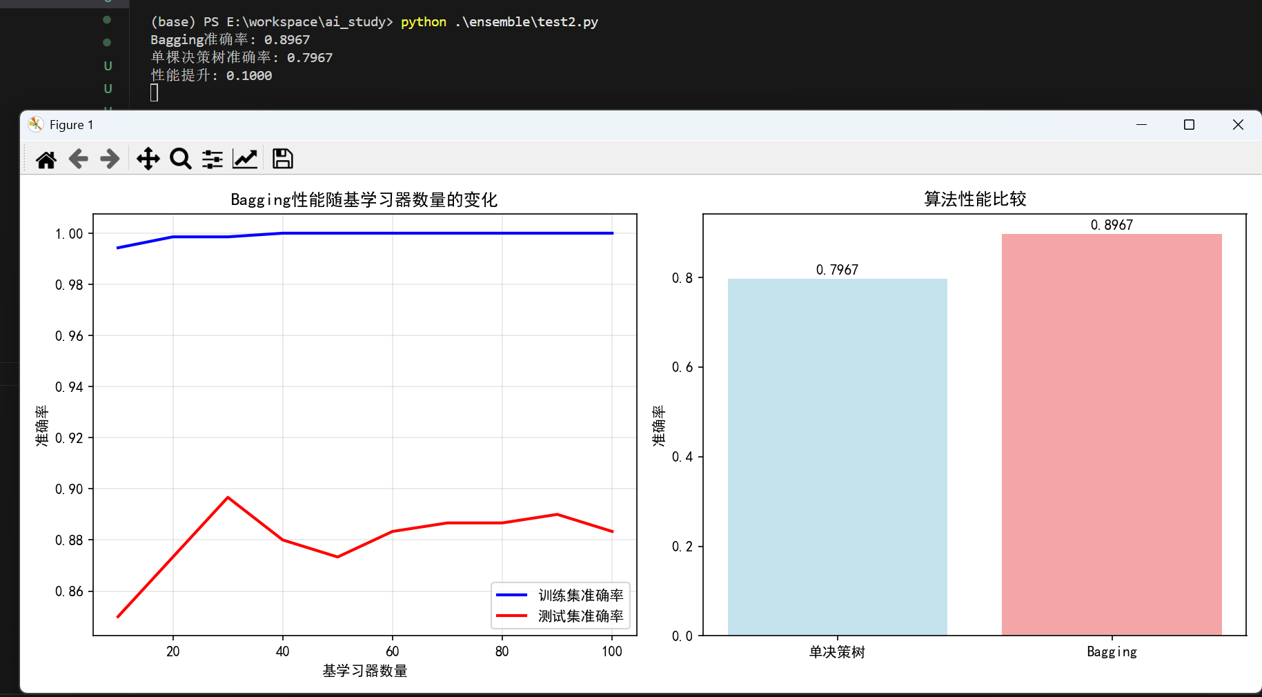
single_accuracy = accuracy_score(y_test, y_pred_single)print(f"Bagging准确率: {bagging_accuracy:.4f}")
print(f"单棵决策树准确率: {single_accuracy:.4f}")
print(f"性能提升: {(bagging_accuracy - single_accuracy):.4f}")# 可视化不同基学习器数量对性能的影响
n_estimators_range = [10, 20, 30, 40, 50, 60, 70, 80, 90, 100]
train_scores = []
test_scores = []for n in n_estimators_range:clf = BaggingClassifier(estimator=DecisionTreeClassifier(),n_estimators=n,random_state=42)clf.fit(X_train, y_train)train_scores.append(accuracy_score(y_train, clf.predict(X_train)))test_scores.append(accuracy_score(y_test, clf.predict(X_test)))plt.figure(figsize=(12, 5))plt.subplot(1, 2, 1)
plt.plot(n_estimators_range, train_scores, 'b-', label='训练集准确率', linewidth=2)
plt.plot(n_estimators_range, test_scores, 'r-', label='测试集准确率', linewidth=2)
plt.xlabel('基学习器数量')
plt.ylabel('准确率')
plt.title('Bagging性能随基学习器数量的变化')
plt.legend()
plt.grid(True, alpha=0.3)plt.subplot(1, 2, 2)
# 比较不同算法的性能
methods = ['单决策树', 'Bagging']
accuracies = [single_accuracy, bagging_accuracy]
colors = ['lightblue', 'lightcoral']plt.bar(methods, accuracies, color=colors, alpha=0.7)
plt.ylabel('准确率')
plt.title('算法性能比较')
for i, v in enumerate(accuracies):plt.text(i, v + 0.01, f'{v:.4f}', ha='center')plt.tight_layout()
plt.show()

运行结果:

Bagging的有效性条件

Bagging在学习器"不稳定"时效果最好：

不稳定学习器：训练集小的差异可以造成产生的假设大不相同
典型代表：决策树、神经网络
稳定学习器（如K近邻）使用Bagging效果提升有限

2.3 Boosting（提升方法）

Boosting方法顺序训练基学习器，每个后续学习器更关注前一个学习器错误分类的样本。

AdaBoost算法详解

AdaBoost（Adaptive Boosting）是最著名的Boosting算法：

算法流程：

初始化样本权重： $w_i = 1/N$ （所有样本权重相等）
对于 $\ldots, T$ ：
- 用当前权重分布训练基学习器 $h_t$
- 计算错误率： $ϵt=∑i=1Nwi⋅I(yi≠ht(xi))\epsilon_t = \sum_{i=1}^N w_i \cdot I(y_i \neq h_t(x_i))$
- 计算学习器权重： $αt=12ln⁡(1−ϵtϵt)\alpha_t = \frac{1}{2} \ln\left(\frac{1-\epsilon_t}{\epsilon_t}\right)$
- 更新样本权重：
  - 正确分类： $winew=wiold⋅e−αtw_i^{\text{new}} = w_i^{\text{old}} \cdot e^{-\alpha_t}$
  - 错误分类： $winew=wiold⋅eαtw_i^{\text{new}} = w_i^{\text{old}} \cdot e^{\alpha_t}$
- 归一化权重（使权重和为1）
最终分类器： $\text{sign}\left(\sum_{t=1}^T \alpha_t h_t(x)\right)$

Python实战示例

from sklearn.ensemble import AdaBoostClassifier
from sklearn.tree import DecisionTreeClassifier
import matplotlib.pyplot as plt
import numpy as np# 创建AdaBoost分类器（使用决策树桩）
adaboost_clf = AdaBoostClassifier(estimator=DecisionTreeClassifier(max_depth=1),  # 弱学习器：决策树桩n_estimators=50,learning_rate=1.0,random_state=42
)# 训练和评估
adaboost_clf.fit(X_train, y_train)
y_pred_adaboost = adaboost_clf.predict(X_test)
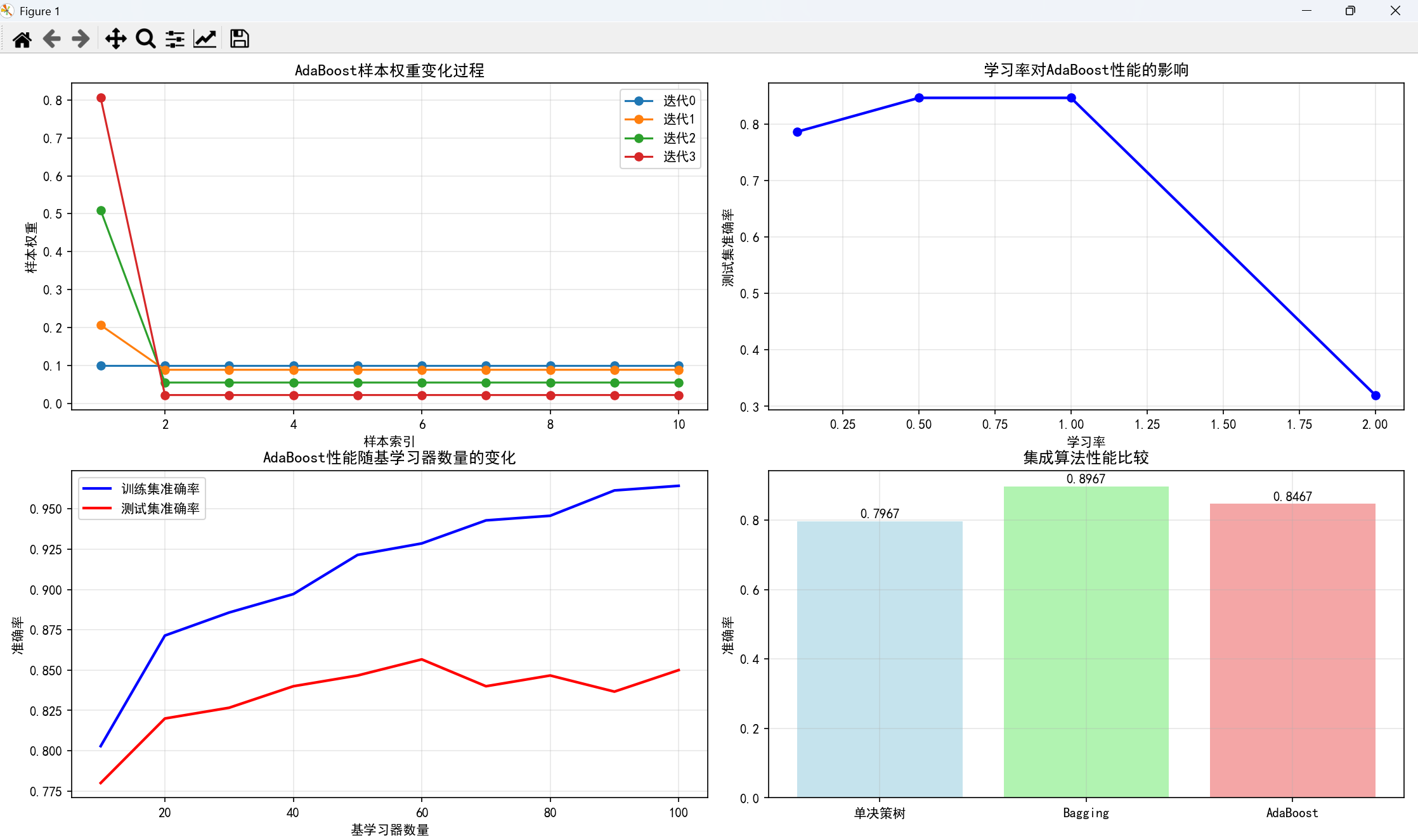
adaboost_accuracy = accuracy_score(y_test, y_pred_adaboost)print(f"AdaBoost准确率: {adaboost_accuracy:.4f}")# 可视化训练过程中样本权重的变化
plt.figure(figsize=(15, 10))# 模拟AdaBoost权重更新过程
def simulate_adaboost_weights(n_samples=10, n_iterations=3):# 初始权重weights = np.ones(n_samples) / n_samplesweight_history = [weights.copy()]for iteration in range(n_iterations):# 模拟错误率（假设第一个样本被错误分类）error_rate = 0.3 if iteration == 0 else 0.2# 计算alphaalpha = 0.5 * np.log((1 - error_rate) / error_rate)# 更新权重（简化版：假设第一个样本错误分类，其他正确）for i in range(n_samples):if i == 0:  # 错误分类weights[i] *= np.exp(alpha)else:       # 正确分类weights[i] *= np.exp(-alpha)# 归一化weights /= np.sum(weights)weight_history.append(weights.copy())return weight_historyweight_history = simulate_adaboost_weights()plt.subplot(2, 2, 1)
for i in range(len(weight_history)):plt.plot(range(1, 11), weight_history[i], marker='o', label=f'迭代{i}')
plt.xlabel('样本索引')
plt.ylabel('样本权重')
plt.title('AdaBoost样本权重变化过程')
plt.legend()
plt.grid(True, alpha=0.3)# 不同学习率的影响
learning_rates = [0.1, 0.5, 1.0, 2.0]
lr_scores = []for lr in learning_rates:clf = AdaBoostClassifier(estimator=DecisionTreeClassifier(max_depth=1),n_estimators=50,learning_rate=lr,random_state=42)clf.fit(X_train, y_train)lr_scores.append(accuracy_score(y_test, clf.predict(X_test)))plt.subplot(2, 2, 2)
plt.plot(learning_rates, lr_scores, 'bo-', linewidth=2)
plt.xlabel('学习率')
plt.ylabel('测试集准确率')
plt.title('学习率对AdaBoost性能的影响')
plt.grid(True, alpha=0.3)# 基学习器数量对性能的影响
n_estimators_list = [10, 20, 30, 40, 50, 60, 70, 80, 90, 100]
ada_train_scores = []
ada_test_scores = []for n in n_estimators_list:clf = AdaBoostClassifier(estimator=DecisionTreeClassifier(max_depth=1),n_estimators=n,random_state=42)clf.fit(X_train, y_train)ada_train_scores.append(accuracy_score(y_train, clf.predict(X_train)))ada_test_scores.append(accuracy_score(y_test, clf.predict(X_test)))plt.subplot(2, 2, 3)
plt.plot(n_estimators_list, ada_train_scores, 'b-', label='训练集准确率', linewidth=2)
plt.plot(n_estimators_list, ada_test_scores, 'r-', label='测试集准确率', linewidth=2)
plt.xlabel('基学习器数量')
plt.ylabel('准确率')
plt.title('AdaBoost性能随基学习器数量的变化')
plt.legend()
plt.grid(True, alpha=0.3)# 算法比较
plt.subplot(2, 2, 4)
algorithms = ['单决策树', 'Bagging', 'AdaBoost']
accuracies = [single_accuracy, bagging_accuracy, adaboost_accuracy]
colors = ['lightblue', 'lightgreen', 'lightcoral']bars = plt.bar(algorithms, accuracies, color=colors, alpha=0.7)
plt.ylabel('准确率')
plt.title('集成算法性能比较')# 添加数值标签
for bar, accuracy in zip(bars, accuracies):plt.text(bar.get_x() + bar.get_width()/2, bar.get_height() + 0.01, f'{accuracy:.4f}', ha='center')plt.grid(True, alpha=0.3)
plt.tight_layout()
plt.show()

执行结果:

AdaBoost的优点与注意事项

优点：

非常快速且易于实现
只有一个主要参数（迭代次数T）需要调节
灵活：可以与任何分类器结合
特别适合弱学习器

注意事项：

性能依赖于数据和弱学习器的选择
在下列情况下可能失效：
- 弱学习器太复杂（容易过拟合）
- 弱学习器太弱（ $αt→0\alpha_t \rightarrow 0$ 太快）
- 数据噪声较大

三、Bagging vs Boosting：核心差异对比

特性	Bagging	Boosting
训练方式	并行训练，各基学习器相互独立	顺序训练，后续学习器依赖前一个
样本权重	所有样本权重相等	动态调整样本权重，关注难样本
基学习器关系	相互独立，可并行化	强依赖，必须顺序训练
对噪声的敏感性	相对不敏感	比较敏感
方差/偏差	主要降低方差	主要降低偏差
适用场景	高方差模型（如深度决策树）	高偏差模型（如决策树桩）

四、进阶集成方法与实践技巧

4.1 随机森林（Random Forest）

随机森林是Bagging的扩展，在构建决策树时不仅对样本采样，还对特征采样。

from sklearn.ensemble import RandomForestClassifier# 创建随机森林分类器
rf_clf = RandomForestClassifier(n_estimators=100,max_depth=10,min_samples_split=2,min_samples_leaf=1,max_features='sqrt',  # 特征采样bootstrap=True,       # 样本采样random_state=42
)rf_clf.fit(X_train, y_train)
rf_accuracy = rf_clf.score(X_test, y_test)
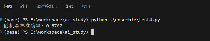
print(f"随机森林准确率: {rf_accuracy:.4f}")

执行结果:

4.2 重新调权 vs 重新采样

在Boosting中，有两种处理样本权重的方式：

重新调权：直接使用样本权重训练基学习器

优点：更精确地反映样本重要性
缺点：需要学习器支持样本权重

重新采样：根据样本权重进行采样

优点：兼容性更好
缺点：引入采样随机性

# 重新采样实现示例
from sklearn.utils import resampledef boosting_resampling(X, y, base_estimator, n_estimators=50):estimators = []alphas = []# 初始权重sample_weights = np.ones(len(X)) / len(X)for t in range(n_estimators):# 根据权重重新采样indices = resample(range(len(X)), replace=True, n_samples=len(X), random_state=42+t, weights=sample_weights)X_resampled = X[indices]y_resampled = y[indices]# 训练基学习器estimator = base_estimator.fit(X_resampled, y_resampled)y_pred = estimator.predict(X)# 计算错误率和alphaerror_mask = (y_pred != y)error_rate = np.sum(sample_weights[error_mask])alpha = 0.5 * np.log((1 - error_rate) / error_rate)# 更新权重sample_weights[~error_mask] *= np.exp(-alpha)  # 正确分类sample_weights[error_mask] *= np.exp(alpha)    # 错误分类sample_weights /= np.sum(sample_weights)       # 归一化estimators.append(estimator)alphas.append(alpha)return estimators, alphas

4.3 集成学习参数调优

from sklearn.model_selection import GridSearchCV# AdaBoost参数调优
param_grid = {'n_estimators': [50, 100, 200],'learning_rate': [0.01, 0.1, 1.0]
}grid_search = GridSearchCV(AdaBoostClassifier(estimator=DecisionTreeClassifier(max_depth=1), algorithm='SAMME'),param_grid,cv=5,scoring='accuracy',n_jobs=-1
)grid_search.fit(X_train, y_train)
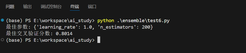
print(f"最佳参数: {grid_search.best_params_}")
print(f"最佳交叉验证分数: {grid_search.best_score_:.4f}")

执行结果:

五、实际应用场景与最佳实践

5.1 适用场景

互联网内容过滤：垃圾邮件检测、内容分类
图像识别：人脸识别、物体检测
手写识别：数字识别、文字识别
语音识别：语音转文本、说话人识别
文本分类：情感分析、主题分类

5.2 最佳实践建议

基学习器选择原则：
- 准确性：每个基学习器至少要比随机猜测好
- 多样性：基学习器之间应该尽可能不同
- 计算效率：考虑训练和预测的时间成本
避免过拟合策略：
- 控制基学习器的复杂度
- 使用交叉验证选择最优参数
- 监控训练和验证集的性能差异
算法选择指南：
- 数据噪声大 → 优先选择Bagging
- 追求最高精度 → 尝试Boosting
- 需要稳定可解释 → 选择随机森林