使用LSTM进行人类活动识别

使用LSTM进行人类活动识别

使用智能手机数据集和LSTM RNN进行人类活动识别(HAR)。在六个类别中对运动类型进行分类：

• 步行(WALKING)
• 上楼(WALKING_UPSTAIRS)
• 下楼(WALKING_DOWNSTAIRS)
• 坐着(SITTING)
• 站立(STANDING)
• 躺着(LAYING)

与经典方法相比，使用带有长短期记忆单元(LSTMs)的循环神经网络(RNN)几乎不需要特征工程。数据可以直接输入到神经网络中，神经网络就像一个黑匣子，能够正确地对问题进行建模。关于活动识别数据集的其它研究使用了大量的特征工程，这更像是信号处理方法与经典数据科学技术的结合。而这里的方法在数据预处理方面非常简单。

让我们使用Google简洁的深度学习库TensorFlow，演示LSTM（一种可以处理序列数据/时间序列的人工神经网络）的使用。

视频数据集概览

点击此链接查看实验中记录的一位参与者执行6项活动的视频：

[观看视频]

关于输入数据的详细信息

我将使用LSTM对数据进行学习（作为系在腰部的手机）来识别用户正在进行的活动类型。数据集的描述如下：

传感器信号（加速度计和陀螺仪）通过应用噪声滤波器进行预处理，然后在2.56秒固定宽度滑动窗口和50%重叠（128个读数/窗口）中进行采样。传感器加速度信号具有重力和身体运动分量，使用巴特沃斯低通滤波器将其分离为身体加速度和重力。假设重力仅具有低频分量，因此使用了截止频率为0.3 Hz的滤波器。

也就是说，我将使用几乎原始的数据：仅作为预处理步骤，将重力影响从加速度计中过滤出来，作为另一个3D特征输入以帮助学习。如果您想自己提取重力，可以分叉我关于在Python中使用巴特沃斯低通滤波器(LPF)的代码，并将其编辑为具有0.3 Hz的正确截止频率，这是从身体传感器进行活动识别的良好频率。

什么是RNN？

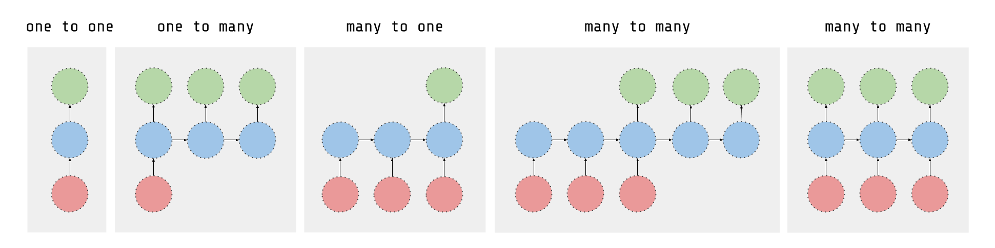
正如这篇文章所解释的，RNN接受多个输入向量进行处理并输出其他向量。可以大致想象成下图所示，想象每个矩形具有矢量深度以及下图中其他特殊的隐藏特性。在我们的例子中，使用了"多对一"架构：我们接受特征向量的时间序列（每个时间步一个向量）将其转换为输出端的概率向量以进行分类。请注意，"一对一"架构将是标准的前馈神经网络。

了解更多关于RNN的信息

什么是LSTM？

LSTM是一种改进的RNN。它更复杂，但更容易训练，避免了所谓的梯度消失问题。我推荐您学习这个课程以了解更多关于LSTM的知识。

了解更多关于LSTM的信息

结果

往下滚动！有漂亮的视觉效果等着您。

# 所有包含的文件import numpy as np
import matplotlib
import matplotlib.pyplot as plt
import tensorflow as tf  # 版本 1.0.0（过去提交中使用了某些早期版本）
from sklearn import metricsimport os

# 有用的常量# 这些是用于神经网络的独立归一化输入特征
INPUT_SIGNAL_TYPES = ["body_acc_x_","body_acc_y_","body_acc_z_","body_gyro_x_","body_gyro_y_","body_gyro_z_","total_acc_x_","total_acc_y_","total_acc_z_"
]# 要学习分类的输出类别
LABELS = ["WALKING","WALKING_UPSTAIRS","WALKING_DOWNSTAIRS","SITTING","STANDING","LAYING"
]

让我们从下载数据开始：

# 注意：在"ipython notebook"单元格中，Linux bash命令以"!"开头DATA_PATH = "data/"!pwd && ls
os.chdir(DATA_PATH)
!pwd && ls!python download_dataset.py!pwd && ls
os.chdir("..")
!pwd && lsDATASET_PATH = DATA_PATH + "UCI HAR Dataset/"
print("\n" + "数据集现在位于: " + DATASET_PATH)

/home/ubuntu/pynb/LSTM-Human-Activity-Recognition
data	 LSTM_files  LSTM_OLD.ipynb  README.md
LICENSE  LSTM.ipynb  lstm.py	     screenlog.0
/home/ubuntu/pynb/LSTM-Human-Activity-Recognition/data
download_dataset.py  source.txtDownloading...
--2017-05-24 01:49:53--  https://archive.ics.uci.edu/ml/machine-learning-databases/00240/UCI%20HAR%20Dataset.zip
Resolving archive.ics.uci.edu (archive.ics.uci.edu)... 128.195.10.249
Connecting to archive.ics.uci.edu (archive.ics.uci.edu)|128.195.10.249|:443... connected.
HTTP request sent, awaiting response... 200 OK
Length: 60999314 (58M) [application/zip]
Saving to: ‘UCI HAR Dataset.zip’100%[======================================>] 60,999,314  1.69MB/s   in 38s    2017-05-24 01:50:31 (1.55 MB/s) - ‘UCI HAR Dataset.zip’ saved [60999314/60999314]Downloading done.Extracting...
Extracting successfully done to /home/ubuntu/pynb/LSTM-Human-Activity-Recognition/data/UCI HAR Dataset.
/home/ubuntu/pynb/LSTM-Human-Activity-Recognition/data
download_dataset.py  __MACOSX  source.txt  UCI HAR Dataset  UCI HAR Dataset.zip
/home/ubuntu/pynb/LSTM-Human-Activity-Recognition
data	 LSTM_files  LSTM_OLD.ipynb  README.md
LICENSE  LSTM.ipynb  lstm.py	     screenlog.0Dataset is now located at: data/UCI HAR Dataset/

准备数据集：

TRAIN = "train/"
TEST = "test/"# 加载"X"（神经网络的训练和测试输入）def load_X(X_signals_paths):X_signals = []for signal_type_path in X_signals_paths:file = open(signal_type_path, 'r')# 从磁盘读取数据集，处理文本文件的语法X_signals.append([np.array(serie, dtype=np.float32) for serie in [row.replace('  ', ' ').strip().split(' ') for row in file]])file.close()return np.transpose(np.array(X_signals), (1, 2, 0))X_train_signals_paths = [DATASET_PATH + TRAIN + "Inertial Signals/" + signal + "train.txt" for signal in INPUT_SIGNAL_TYPES
]
X_test_signals_paths = [DATASET_PATH + TEST + "Inertial Signals/" + signal + "test.txt" for signal in INPUT_SIGNAL_TYPES
]X_train = load_X(X_train_signals_paths)
X_test = load_X(X_test_signals_paths)# 加载"y"（神经网络的训练和测试输出）def load_y(y_path):file = open(y_path, 'r')# 从磁盘读取数据集，处理文本文件的语法y_ = np.array([elem for elem in [row.replace('  ', ' ').strip().split(' ') for row in file]],dtype=np.int32)file.close()# 为每个输出类减去1以进行友好的基于0的索引return y_ - 1y_train_path = DATASET_PATH + TRAIN + "y_train.txt"
y_test_path = DATASET_PATH + TEST + "y_test.txt"y_train = load_y(y_train_path)
y_test = load_y(y_test_path)

附加参数：

以下是训练的一些核心参数定义。

例如，整个神经网络的结构可以通过枚举这些参数以及两个LSTM在时间步上作为隐藏层一个堆叠在另一个（堆叠）输出到输入的事实来总结。

# 输入数据training_data_count = len(X_train)  # 7352个训练序列（每个序列之间有50%的重叠）
test_data_count = len(X_test)  # 2947个测试序列
n_steps = len(X_train[0])  # 每个序列128个时间步
n_input = len(X_train[0][0])  # 每个时间步9个输入参数# LSTM神经网络的内部结构n_hidden = 32 # 隐藏层特征数
n_classes = 6 # 总类别数（应该增加或减少）# 训练learning_rate = 0.0025
lambda_loss_amount = 0.0015
training_iters = training_data_count * 300  # 在数据集上循环300次
batch_size = 1500
display_iter = 30000  # 在训练期间显示测试集准确率# 一些调试信息print("一些有用的信息，用于了解数据集的形状和归一化情况：")
print("(X形状, y形状, 每个X的均值, 每个X的标准差)")
print(X_test.shape, y_test.shape, np.mean(X_test), np.std(X_test))
print("因此数据集如预期那样正确归一化，但尚未进行独热编码。")

Some useful info to get an insight on dataset's shape and normalisation:
(X shape, y shape, every X's mean, every X's standard deviation)
(2947, 128, 9) (2947, 1) 0.0991399 0.395671
The dataset is therefore properly normalised, as expected, but not yet one-hot encoded.

用于训练的实用函数：

def LSTM_RNN(_X, _weights, _biases):# 该函数根据给定参数返回一个TensorFlow LSTM (RNN) 人工神经网络。# 此外，堆叠了两个LSTM单元，这增加了神经网络的深度。# 注意，本笔记本中的一些代码灵感来自在另一个数据集上使用的略有不同的RNN架构，部分功劳归于"aymericdamien"（MIT许可）。# （注意：通过一次性塑造数据集可以大大优化此步骤）# 输入形状: (batch_size, n_steps, n_input)_X = tf.transpose(_X, [1, 0, 2])  # 置换n_steps和batch_size# 重塑以准备输入到隐藏层激活_X = tf.reshape(_X, [-1, n_input])# 新形状: (n_steps*batch_size, n_input)# ReLU激活，感谢Yu Zhao在此处添加此改进：_X = tf.nn.relu(tf.matmul(_X, _weights['hidden']) + _biases['hidden'])# 分割数据，因为RNN单元需要输入列表以供RNN内部循环使用_X = tf.split(_X, n_steps, 0)# 新形状: n_steps * (batch_size, n_hidden)# 使用TensorFlow定义两个堆叠的LSTM单元（两个循环层深度）lstm_cell_1 = tf.contrib.rnn.BasicLSTMCell(n_hidden, forget_bias=1.0, state_is_tuple=True)lstm_cell_2 = tf.contrib.rnn.BasicLSTMCell(n_hidden, forget_bias=1.0, state_is_tuple=True)lstm_cells = tf.contrib.rnn.MultiRNNCell([lstm_cell_1, lstm_cell_2], state_is_tuple=True)# 获取LSTM单元输出outputs, states = tf.contrib.rnn.static_rnn(lstm_cells, _X, dtype=tf.float32)# 对于"多对一"风格的分类器，获取最后一个时间步的输出特征，# 如本页顶部描述RNN的图像所示lstm_last_output = outputs[-1]# 线性激活return tf.matmul(lstm_last_output, _weights['out']) + _biases['out']def extract_batch_size(_train, step, batch_size):# 从"(X|y)_train"数据中获取"batch_size"数量的数据的函数。shape = list(_train.shape)shape[0] = batch_sizebatch_s = np.empty(shape)for i in range(batch_size):# 循环索引index = ((step-1)*batch_size + i) % len(_train)batch_s[i] = _train[index]return batch_sdef one_hot(y_, n_classes=n_classes):# 从数字索引编码神经网络的独热输出标签的函数# 例如：# one_hot(y_=[[5], [0], [3]], n_classes=6):#     返回 [[0, 0, 0, 0, 0, 1], [1, 0, 0, 0, 0, 0], [0, 0, 0, 1, 0, 0]]y_ = y_.reshape(len(y_))return np.eye(n_classes)[np.array(y_, dtype=np.int32)]  # 返回浮点数

让我们认真起来，构建神经网络：

# 图输入/输出
x = tf.placeholder(tf.float32, [None, n_steps, n_input])
y = tf.placeholder(tf.float32, [None, n_classes])# 图权重
weights = {'hidden': tf.Variable(tf.random_normal([n_input, n_hidden])), # 隐藏层权重'out': tf.Variable(tf.random_normal([n_hidden, n_classes], mean=1.0))
}
biases = {'hidden': tf.Variable(tf.random_normal([n_hidden])),'out': tf.Variable(tf.random_normal([n_classes]))
}pred = LSTM_RNN(x, weights, biases)# 损失、优化器和评估
l2 = lambda_loss_amount * sum(tf.nn.l2_loss(tf_var) for tf_var in tf.trainable_variables()
) # L2损失防止这个过度的神经网络对数据过拟合
cost = tf.reduce_mean(tf.nn.softmax_cross_entropy_with_logits(labels=y, logits=pred)) + l2 # Softmax损失
optimizer = tf.train.AdamOptimizer(learning_rate=learning_rate).minimize(cost) # Adam优化器correct_pred = tf.equal(tf.argmax(pred,1), tf.argmax(y,1))
accuracy = tf.reduce_mean(tf.cast(correct_pred, tf.float32))

好极了，现在训练神经网络：

# 记录训练性能
test_losses = []
test_accuracies = []
train_losses = []
train_accuracies = []# 启动图
sess = tf.InteractiveSession(config=tf.ConfigProto(log_device_placement=True))
init = tf.global_variables_initializer()
sess.run(init)# 在每个循环中使用"batch_size"数量的示例数据执行训练步骤
step = 1
while step * batch_size <= training_iters:batch_xs =         extract_batch_size(X_train, step, batch_size)batch_ys = one_hot(extract_batch_size(y_train, step, batch_size))# 使用批量数据进行训练_, loss, acc = sess.run([optimizer, cost, accuracy],feed_dict={x: batch_xs,y: batch_ys})train_losses.append(loss)train_accuracies.append(acc)# 仅在某些步骤评估网络以加快训练速度：if (step*batch_size % display_iter == 0) or (step == 1) or (step * batch_size > training_iters):# 为了不刷屏，在此"if"中显示训练准确率/损失print("训练迭代 #" + str(step*batch_size) + \":   批量损失 = " + "{:.6f}".format(loss) + \", 准确率 = {}".format(acc))# 在测试集上进行评估（此处不进行学习 - 仅用于诊断的评估）loss, acc = sess.run([cost, accuracy],feed_dict={x: X_test,y: one_hot(y_test)})test_losses.append(loss)test_accuracies.append(acc)print("测试集表现: " + \"批量损失 = {}".format(loss) + \", 准确率 = {}".format(acc))step += 1print("优化完成！")# 测试数据的准确率one_hot_predictions, accuracy, final_loss = sess.run([pred, accuracy, cost],feed_dict={x: X_test,y: one_hot(y_test)}
)test_losses.append(final_loss)
test_accuracies.append(accuracy)print("最终结果: " + \"批量损失 = {}".format(final_loss) + \", 准确率 = {}".format(accuracy))

WARNING:tensorflow:From <ipython-input-19-3339689e51f6>:9: initialize_all_variables (from tensorflow.python.ops.variables) is deprecated and will be removed after 2017-03-02.
Instructions for updating:
Use `tf.global_variables_initializer` instead.
Training iter #1500:   Batch Loss = 5.416760, Accuracy = 0.15266665816307068
PERFORMANCE ON TEST SET: Batch Loss = 4.880829811096191, Accuracy = 0.05632847175002098
Training iter #30000:   Batch Loss = 3.031930, Accuracy = 0.607333242893219
PERFORMANCE ON TEST SET: Batch Loss = 3.0515167713165283, Accuracy = 0.6067186594009399
Training iter #60000:   Batch Loss = 2.672764, Accuracy = 0.7386666536331177
PERFORMANCE ON TEST SET: Batch Loss = 2.780435085296631, Accuracy = 0.7027485370635986
Training iter #90000:   Batch Loss = 2.378301, Accuracy = 0.8366667032241821
PERFORMANCE ON TEST SET: Batch Loss = 2.6019773483276367, Accuracy = 0.7617915868759155
Training iter #120000:   Batch Loss = 2.127290, Accuracy = 0.9066667556762695
PERFORMANCE ON TEST SET: Batch Loss = 2.3625404834747314, Accuracy = 0.8116728663444519
Training iter #150000:   Batch Loss = 1.929805, Accuracy = 0.9380000233650208
PERFORMANCE ON TEST SET: Batch Loss = 2.306251049041748, Accuracy = 0.8276212215423584
Training iter #180000:   Batch Loss = 1.971904, Accuracy = 0.9153333902359009
PERFORMANCE ON TEST SET: Batch Loss = 2.0835530757904053, Accuracy = 0.8771631121635437
Training iter #210000:   Batch Loss = 1.860249, Accuracy = 0.8613333702087402
PERFORMANCE ON TEST SET: Batch Loss = 1.9994492530822754, Accuracy = 0.8788597583770752
Training iter #240000:   Batch Loss = 1.626292, Accuracy = 0.9380000233650208
PERFORMANCE ON TEST SET: Batch Loss = 1.879166603088379, Accuracy = 0.8944689035415649
Training iter #270000:   Batch Loss = 1.582758, Accuracy = 0.9386667013168335
PERFORMANCE ON TEST SET: Batch Loss = 2.0341007709503174, Accuracy = 0.8361043930053711
Training iter #300000:   Batch Loss = 1.620352, Accuracy = 0.9306666851043701
PERFORMANCE ON TEST SET: Batch Loss = 1.8185184001922607, Accuracy = 0.8639293313026428
Training iter #330000:   Batch Loss = 1.474394, Accuracy = 0.9693333506584167
PERFORMANCE ON TEST SET: Batch Loss = 1.7638503313064575, Accuracy = 0.8747878670692444
Training iter #360000:   Batch Loss = 1.406998, Accuracy = 0.9420000314712524
PERFORMANCE ON TEST SET: Batch Loss = 1.5946787595748901, Accuracy = 0.902273416519165
Training iter #390000:   Batch Loss = 1.362515, Accuracy = 0.940000057220459
PERFORMANCE ON TEST SET: Batch Loss = 1.5285792350769043, Accuracy = 0.9046487212181091
Training iter #420000:   Batch Loss = 1.252860, Accuracy = 0.9566667079925537
PERFORMANCE ON TEST SET: Batch Loss = 1.4635565280914307, Accuracy = 0.9107565879821777
Training iter #450000:   Batch Loss = 1.190078, Accuracy = 0.9553333520889282
...
PERFORMANCE ON TEST SET: Batch Loss = 0.42567864060401917, Accuracy = 0.9324736595153809
Training iter #2070000:   Batch Loss = 0.342763, Accuracy = 0.9326667189598083
PERFORMANCE ON TEST SET: Batch Loss = 0.4292983412742615, Accuracy = 0.9273836612701416
Training iter #2100000:   Batch Loss = 0.259442, Accuracy = 0.9873334169387817
PERFORMANCE ON TEST SET: Batch Loss = 0.44131210446357727, Accuracy = 0.9273836612701416
Training iter #2130000:   Batch Loss = 0.284630, Accuracy = 0.9593333601951599
PERFORMANCE ON TEST SET: Batch Loss = 0.46982717514038086, Accuracy = 0.9093992710113525
Training iter #2160000:   Batch Loss = 0.299012, Accuracy = 0.9686667323112488
PERFORMANCE ON TEST SET: Batch Loss = 0.48389002680778503, Accuracy = 0.9138105511665344
Training iter #2190000:   Batch Loss = 0.287106, Accuracy = 0.9700000286102295
PERFORMANCE ON TEST SET: Batch Loss = 0.4670214056968689, Accuracy = 0.9216151237487793
Optimization Finished!
FINAL RESULT: Batch Loss = 0.45611169934272766, Accuracy = 0.9165252447128296

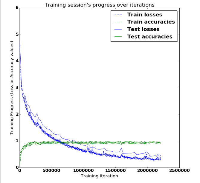
训练是好的，但有视觉洞察力更好：

好的，现在让我们在笔记本中简单地绘制这个。

# (Inline plots: )
%matplotlib inlinefont = {'family' : 'Bitstream Vera Sans','weight' : 'bold','size'   : 18
}
matplotlib.rc('font', **font)width = 12
height = 12
plt.figure(figsize=(width, height))indep_train_axis = np.array(range(batch_size, (len(train_losses)+1)*batch_size, batch_size))
plt.plot(indep_train_axis, np.array(train_losses),     "b--", label="Train losses")
plt.plot(indep_train_axis, np.array(train_accuracies), "g--", label="Train accuracies")indep_test_axis = np.append(np.array(range(batch_size, len(test_losses)*display_iter, display_iter)[:-1]),[training_iters]
)
plt.plot(indep_test_axis, np.array(test_losses),     "b-", label="Test losses")
plt.plot(indep_test_axis, np.array(test_accuracies), "g-", label="Test accuracies")plt.title("Training session's progress over iterations")
plt.legend(loc='upper right', shadow=True)
plt.ylabel('Training Progress (Loss or Accuracy values)')
plt.xlabel('Training iteration')plt.show()

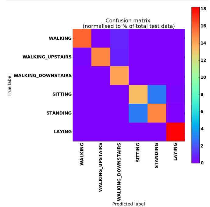
最后是多类别混淆矩阵和指标！

# Resultspredictions = one_hot_predictions.argmax(1)print("Testing Accuracy: {}%".format(100*accuracy))print("")
print("Precision: {}%".format(100*metrics.precision_score(y_test, predictions, average="weighted")))
print("Recall: {}%".format(100*metrics.recall_score(y_test, predictions, average="weighted")))
print("f1_score: {}%".format(100*metrics.f1_score(y_test, predictions, average="weighted")))print("")
print("Confusion Matrix:")
confusion_matrix = metrics.confusion_matrix(y_test, predictions)
print(confusion_matrix)
normalised_confusion_matrix = np.array(confusion_matrix, dtype=np.float32)/np.sum(confusion_matrix)*100print("")
print("Confusion matrix (normalised to % of total test data):")
print(normalised_confusion_matrix)
print("Note: training and testing data is not equally distributed amongst classes, ")
print("so it is normal that more than a 6th of the data is correctly classifier in the last category.")# Plot Results:
width = 12
height = 12
plt.figure(figsize=(width, height))
plt.imshow(normalised_confusion_matrix,interpolation='nearest',cmap=plt.cm.rainbow
)
plt.title("Confusion matrix \n(normalised to % of total test data)")
plt.colorbar()
tick_marks = np.arange(n_classes)
plt.xticks(tick_marks, LABELS, rotation=90)
plt.yticks(tick_marks, LABELS)
plt.tight_layout()
plt.ylabel('True label')
plt.xlabel('Predicted label')
plt.show()

Testing Accuracy: 91.65252447128296%Precision: 91.76286479743305%
Recall: 91.65252799457076%
f1_score: 91.6437546304815%Confusion Matrix:
[[466   2  26   0   2   0][  5 441  25   0   0   0][  1   0 419   0   0   0][  1   1   0 396  87   6][  2   1   0  87 442   0][  0   0   0   0   0 537]]Confusion matrix (normalised to % of total test data):
[[ 15.81269073   0.06786563   0.88225317   0.           0.06786563   0.        ][  0.16966406  14.96437073   0.84832031   0.           0.           0.        ][  0.03393281   0.          14.21784878   0.           0.           0.        ][  0.03393281   0.03393281   0.          13.43739319   2.952154640.20359688][  0.06786563   0.03393281   0.           2.95215464  14.99830341   0.        ][  0.           0.           0.           0.           0.          18.22192001]]
Note: training and testing data is not equally distributed amongst classes,
so it is normal that more than a 6th of the data is correctly classifier in the last category.

sess.close()

结论

非常出色的是，最终准确率达到了91%！并且在训练过程中，根据神经网络权重在训练开始时随机初始化的方式，有时运气好时可以达到93.25%的峰值。

这意味着神经网络几乎总是能够正确识别运动类型！请记住，手机系在腰部，每个要分类的序列仅有两个内部传感器的128个样本窗口（即50 FPS下的2.56秒），因此考虑到这种小的上下文窗口和原始数据，这些预测的准确性令我感到惊讶。我已经验证并重新验证了没有重要的错误，并且社区大量使用和尝试了此代码。

我特别没有预料到在区分"坐着"和"站立"标签方面会有如此好的结果。根据数据集最初收集的方式，从放置在腰部水平的设备的角度来看，这些几乎是相同的事情。不过，仍然可以在这些类别之间的矩阵上看到一个小簇，它只是与对角线略有偏离。这很棒。

还可以看到在区分"步行"、"上楼"和"下楼"方面有些困难。显然，这些活动在运动方面非常相似。

我还尝试了不使用陀螺仪，仅使用3D加速度计的6个特征（并且不更改训练超参数），得到了87%的准确率。通常，陀螺仪比加速度计消耗更多功率，因此最好关闭它们。