DAY 34 GPU训练及类的call方法-

知识点回顾：

CPU性能的查看：看架构代际、核心数、线程数
GPU性能的查看：看显存、看级别、看架构代际
GPU训练的方法：数据和模型移动到GPU device上
类的call方法：为什么定义前向传播时可以直接写作self.fc1(x)
ps：在训练过程中可以在命令行输入nvida-smi查看显存占用情况

import torch
import torch.nn as nn
import torch.optim as optim
from sklearn.datasets import load_iris
from sklearn.model_selection import train_test_split
import numpy as np# 仍然用4特征，3分类的鸢尾花数据集作为我们今天的数据集
# 加载鸢尾花数据集
iris = load_iris()
X = iris.data  # 特征数据
y = iris.target  # 标签数据
# 划分训练集和测试集
X_train, X_test, y_train, y_test = train_test_split(X, y, test_size=0.2, random_state=42)# # 打印下尺寸
# print(X_train.shape)
# print(y_train.shape)
# print(X_test.shape)
# print(y_test.shape)# 归一化数据，神经网络对于输入数据的尺寸敏感，归一化是最常见的处理方式
from sklearn.preprocessing import MinMaxScaler
scaler = MinMaxScaler()
X_train = scaler.fit_transform(X_train)
X_test = scaler.transform(X_test) #确保训练集和测试集是相同的缩放# 将数据转换为 PyTorch 张量，因为 PyTorch 使用张量进行训练
# y_train和y_test是整数，所以需要转化为long类型，如果是float32，会输出1.0 0.0
X_train = torch.FloatTensor(X_train)
y_train = torch.LongTensor(y_train)
X_test = torch.FloatTensor(X_test)
y_test = torch.LongTensor(y_test)class MLP(nn.Module): # 定义一个多层感知机（MLP）模型，继承父类nn.Moduledef __init__(self): # 初始化函数super(MLP, self).__init__() # 调用父类的初始化函数# 前三行是八股文，后面的是自定义的self.fc1 = nn.Linear(4, 10)  # 输入层到隐藏层self.relu = nn.ReLU()self.fc2 = nn.Linear(10, 3)  # 隐藏层到输出层
# 输出层不需要激活函数，因为后面会用到交叉熵函数cross_entropy，交叉熵函数内部有softmax函数，会把输出转化为概率def forward(self, x):out = self.fc1(x)out = self.relu(out)out = self.fc2(out)return out# 实例化模型
model = MLP()# 分类问题使用交叉熵损失函数
criterion = nn.CrossEntropyLoss()# 使用随机梯度下降优化器
optimizer = optim.SGD(model.parameters(), lr=0.01)# # 使用自适应学习率的化器
# optimizer = optim.Adam(model.parameters(), lr=0.001)# 训练模型
num_epochs = 20000 # 训练的轮数# 用于存储每个 epoch 的损失值
losses = []import time
start_time = time.time() # 记录开始时间for epoch in range(num_epochs): # range是从0开始，所以epoch是从0开始# 前向传播outputs = model.forward(X_train)   # 显式调用forward函数# outputs = model(X_train)  # 常见写法隐式调用forward函数，其实是用了model类的__call__方法loss = criterion(outputs, y_train) # output是模型预测值，y_train是真实标签# 反向传播和优化optimizer.zero_grad() #梯度清零，因为PyTorch会累积梯度，所以每次迭代需要清零，梯度累计是那种小的bitchsize模拟大的bitchsizeloss.backward() # 反向传播计算梯度optimizer.step() # 更新参数# 记录损失值losses.append(loss.item())# 打印训练信息if (epoch + 1) % 100 == 0: # range是从0开始，所以epoch+1是从当前epoch开始，每100个epoch打印一次print(f'Epoch [{epoch+1}/{num_epochs}], Loss: {loss.item():.4f}')time_all = time.time() - start_time # 计算训练时间
print(f'Training time: {time_all:.2f} seconds')
import matplotlib.pyplot as plt
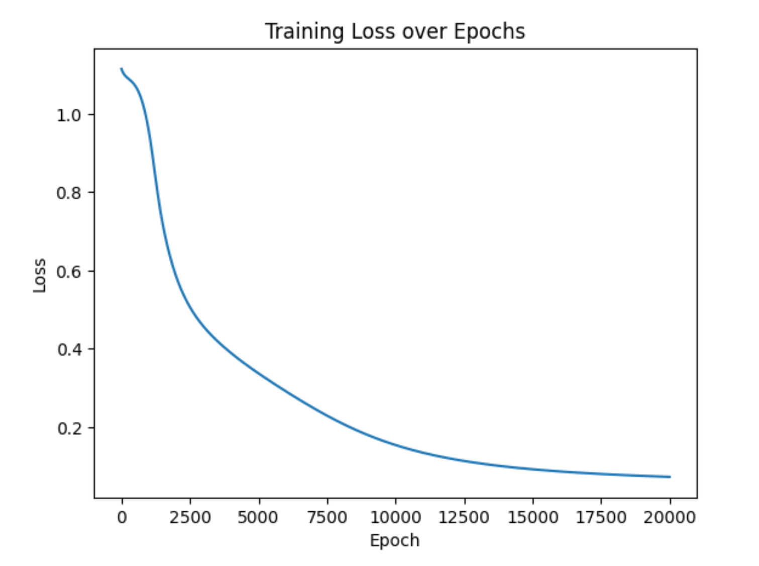
# 可视化损失曲线
plt.plot(range(num_epochs), losses)
plt.xlabel('Epoch')
plt.ylabel('Loss')
plt.title('Training Loss over Epochs')
plt.show()

import wmic = wmi.WMI()
processors = c.Win32_Processor()for processor in processors:print(f"CPU 型号: {processor.Name}")print(f"核心数: {processor.NumberOfCores}")print(f"线程数: {processor.NumberOfLogicalProcessors}")

# 不带参数的call方法
class Counter:def __init__(self):self.count = 0def __call__(self):self.count += 1return self.count# 使用示例
counter = Counter()
print(counter())  # 输出: 1
print(counter())  # 输出: 2
print(counter())
print(counter.count)  # 输出: 2