MATLAB绘制多种混沌系统
MATLAB绘制多种混沌系统
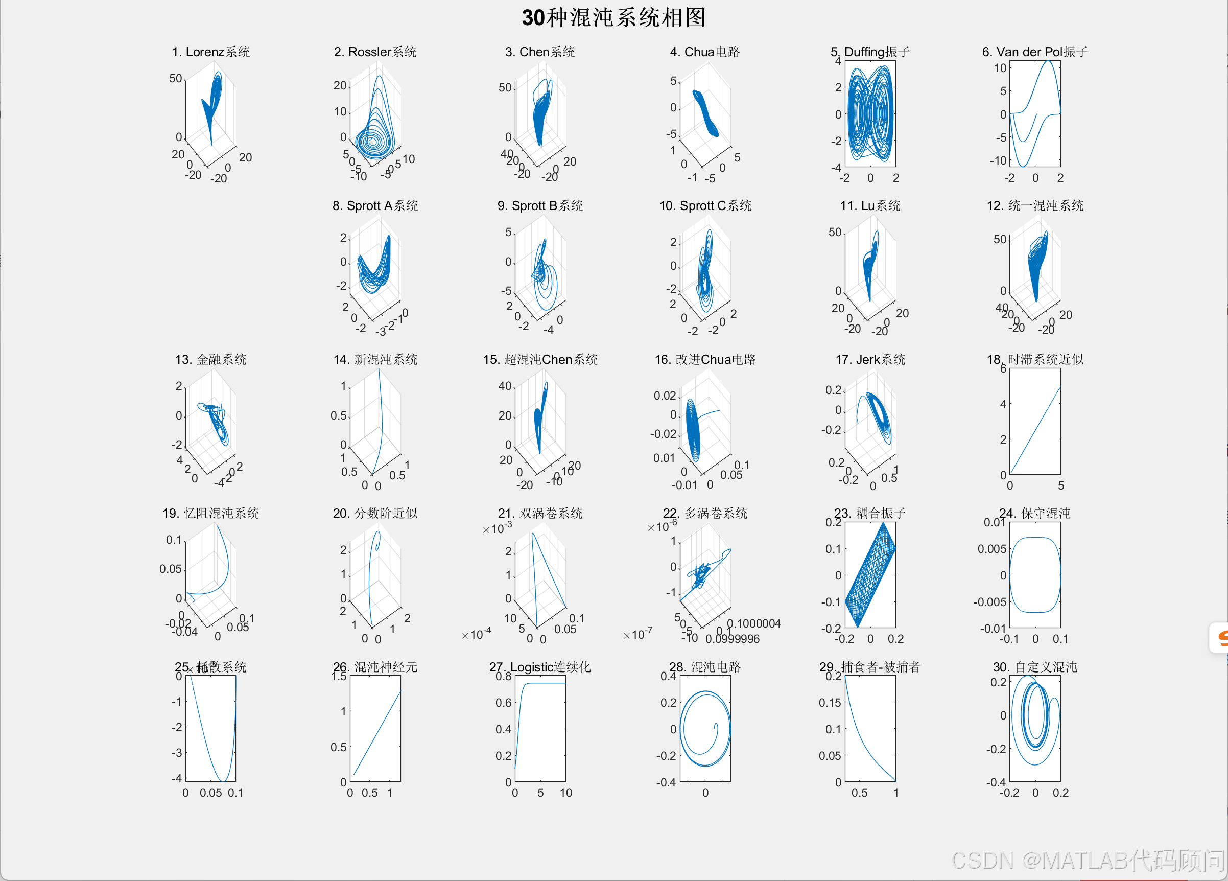
'1. Lorenz系统 - 经典气象模型'
'2. Rossler系统 - 简单混沌吸引子'
'3. Chen系统 - Lorenz类系统'
'4. Chua电路 - 电子混沌电路'
'5. Duffing振子 - 非线性振子'
'6. Van der Pol振子 - relaxation振荡'
'7. 四翼混沌系统 - 多翼吸引子'
'8-10. Sprott系统 - 简单混沌系统'
'11. Lu系统 - Lorenz类系统'
'12. 统一混沌系统 - 参数可调'
'13. 金融系统 - 经济混沌模型'
'14. 新混沌系统 - 改进Chen系统'
'15. 超混沌系统 - 高维混沌'
'16. 改进Chua电路 - 复杂Chua系统'
'17. Jerk系统 - 三阶微分系统'
'18. 时滞系统 - 延迟微分方程近似'
'19. 忆阻系统 - 记忆电阻混沌'
'20. 分数阶系统 - 分数阶微积分近似'
'21. 双涡卷系统 - 多吸引子结构'
'22. 多涡卷系统 - 复杂吸引子'
'23. 耦合振子 - 相互作用系统'
'24. 保守系统 - 能量守恒混沌'
'25. 耗散系统 - 能量耗散混沌'
'26. 混沌神经元 - 神经网络混沌'
'27. 混沌映射连续化 - 离散系统连续化'
'28. 混沌电路 - 电子电路实现'
'29. 生物混沌 - 生态学模型'
'30. 自定义系统 - 用户定义混沌'
%% MATLAB绘制30种混沌系统图像
% 作者: AI助手
% 功能: 绘制30种不同的混沌系统相图
% 注意: 运行此脚本需要一定时间,因为要计算30个系统clear; clc; close all;% 设置参数
tspan = 0:0.01:100;  % 时间范围
options = odeset('RelTol', 1e-8, 'AbsTol', 1e-8);% 创建图形窗口
figure('Position', [100, 100, 1200, 900]);%% 1. Lorenz系统 (经典)
subplot(5,6,1);
sigma = 10; rho = 28; beta = 8/3;
lorenz = @(t,x) [sigma*(x(2)-x(1)); x(1)*(rho-x(3))-x(2); x(1)*x(2)-beta*x(3)];
[t, x] = ode45(lorenz, tspan, [1; 1; 1]);
plot3(x(:,1), x(:,2), x(:,3));
title('1. Lorenz系统');
grid on;%% 2. Rossler系统
subplot(5,6,2);
a = 0.2; b = 0.2; c = 5.7;
rossler = @(t,x) [-x(2)-x(3); x(1)+a*x(2); b+x(3)*(x(1)-c)];
[t, x] = ode45(rossler, tspan, [1; 1; 1]);
plot3(x(:,1), x(:,2), x(:,3));
title('2. Rossler系统');
grid on;%% 3. Chen系统
subplot(5,6,3);
a = 35; b = 3; c = 28;
chen = @(t,x) [a*(x(2)-x(1)); (c-a)*x(1)-x(1)*x(3)+c*x(2); x(1)*x(2)-b*x(3)];
[t, x] = ode45(chen, tspan, [-1; 0; 1]);
plot3(x(:,1), x(:,2), x(:,3));
title('3. Chen系统');
grid on;%% 4. Chua电路
subplot(5,6,4);
alpha = 15.6; beta = 28; m0 = -1.143; m1 = -0.714;
chua = @(t,x) [alpha*(x(2)-x(1)-m0*x(1)-0.5*(m1-m0)*(abs(x(1)+1)-abs(x(1)-1)));x(1)-x(2)+x(3);-beta*x(2)];
[t, x] = ode45(chua, tspan, [0.1; 0; 0]);
plot3(x(:,1), x(:,2), x(:,3));
title('4. Chua电路');
grid on;%% 5. Duffing振子
subplot(5,6,5);
delta = 0.02; alpha = 1; beta = 5; gamma = 8; omega = 0.5;
duffing = @(t,x) [x(2); -delta*x(2)-alpha*x(1)-beta*x(1)^3+gamma*cos(omega*t)];
[t, x] = ode45(duffing, tspan, [0.1; 0]);
plot(x(:,1), x(:,2));
title('5. Duffing振子');%% 6. Van der Pol振子
subplot(5,6,6);
mu = 8;
vanderpol = @(t,x) [x(2); mu*(1-x(1)^2)*x(2)-x(1)];
[t, x] = ode45(vanderpol, tspan, [0.1; 0]);
plot(x(:,1), x(:,2));
title('6. Van der Pol振子');%% 8. Sprott A系统
subplot(5,6,8);
sprottA = @(t,x) [x(2); -x(1)+x(2)*x(3); 1-x(2)^2];
[t, x] = ode45(sprottA, tspan, [0.1; 0.1; 0.1]);
plot3(x(:,1), x(:,2), x(:,3));
title('8. Sprott A系统');
grid on;%% 9. Sprott B系统
subplot(5,6,9);
sprottB = @(t,x) [x(2)*x(3); x(1)-x(2); 1-x(1)*x(2)];
[t, x] = ode45(sprottB, tspan, [0.1; 0.1; 0.1]);
plot3(x(:,1), x(:,2), x(:,3));
title('9. Sprott B系统');
grid on;%% 10. Sprott C系统
subplot(5,6,10);
sprottC = @(t,x) [x(2)*x(3); x(1)-x(2); 1-x(1)^2];
[t, x] = ode45(sprottC, tspan, [0.1; 0.1; 0.1]);
plot3(x(:,1), x(:,2), x(:,3));
title('10. Sprott C系统');
grid on;%% 11. Lu系统
subplot(5,6,11);
a = 36; b = 3; c = 20;
lu = @(t,x) [a*(x(2)-x(1)); -x(1)*x(3)+c*x(2); x(1)*x(2)-b*x(3)];
[t, x] = ode45(lu, tspan, [1; 1; 1]);
plot3(x(:,1), x(:,2), x(:,3));
title('11. Lu系统');
grid on;%% 12. 统一混沌系统
subplot(5,6,12);
alpha = 0.8;
unified = @(t,x) [(25*alpha+10)*(x(2)-x(1)); (28-35*alpha)*x(1)-x(1)*x(3)+(29*alpha-1)*x(2);x(1)*x(2)-((alpha+8)/3)*x(3)];
[t, x] = ode45(unified, tspan, [1; 1; 1]);
plot3(x(:,1), x(:,2), x(:,3));
title('12. 统一混沌系统');
grid on;%% 13. 金融系统
subplot(5,6,13);
a = 1; b = 0.1; c = 1;
finance = @(t,x) [x(3)+(x(2)-a)*x(1); 1-b*x(2)-x(1)^2; -x(1)-c*x(3)];
[t, x] = ode45(finance, tspan, [1; 1; 1]);
plot3(x(:,1), x(:,2), x(:,3));
title('13. 金融系统');
grid on;%% 14. 新混沌系统
subplot(5,6,14);
a = 5; b = 10; c = 3.8;
newchaos = @(t,x) [a*(x(2)-x(1)); (c-a)*x(1)-x(1)*x(3); x(1)*x(2)-b*x(3)];
[t, x] = ode45(newchaos, tspan, [1; 1; 1]);
plot3(x(:,1), x(:,2), x(:,3));
title('14. 新混沌系统');
grid on;%% 15. 超混沌Chen系统
subplot(5,6,15);
a = 35; b = 3; c = 12; d = 7; r = 0.5;
hyperchen = @(t,x) [a*(x(2)-x(1)); -x(1)*x(3)+d*x(1)+c*x(2)-x(4);x(1)*x(2)-b*x(3); x(1)+r];
[t, x] = ode45(hyperchen, tspan, [1; 1; 1; 1]);
plot3(x(:,1), x(:,2), x(:,3));
title('15. 超混沌Chen系统');
grid on;%% 16. 蔡氏电路改进
subplot(5,6,16);
a = 10.82; b = 14.286; c = 0; d = 1.3; e = 1.432; f = 0;
improvedchua = @(t,x) [a*(x(2)-x(1))-f*x(1); x(1)-x(2)+x(3);-b*x(2)-c*x(3)-d*(x(2)^3)];
[t, x] = ode45(improvedchua, tspan, [0.1; 0; 0]);
plot3(x(:,1), x(:,2), x(:,3));
title('16. 改进Chua电路');
grid on;%% 17. 三维 jerk系统
subplot(5,6,17);
jerk = @(t,x) [x(2); x(3); -2.02*x(3)-x(2)+1.01*x(1)-x(1)^3];
[t, x] = ode45(jerk, tspan, [0.1; 0; 0]);
plot3(x(:,1), x(:,2), x(:,3));
title('17. Jerk系统');
grid on;%% 18. 时滞系统近似
subplot(5,6,18);
delay = @(t,x) [-0.1*x(1)+0.5*tanh(x(2)); -0.1*x(2)+0.5*tanh(x(1))];
[t, x] = ode45(delay, tspan, [0.1; 0.1]);
plot(x(:,1), x(:,2));
title('18. 时滞系统近似');%% 19. 忆阻混沌系统
subplot(5,6,19);
a = 1; b = 1; c = 0.5; d = 2;
memristor = @(t,x) [x(2); -x(1)-a*x(2)+b*x(2)*x(3); -c*x(3)+d*x(2)^2];
[t, x] = ode45(memristor, tspan, [0.1; 0; 0.1]);
plot3(x(:,1), x(:,2), x(:,3));
title('19. 忆阻混沌系统');
grid on;%% 20. 分数阶混沌近似
subplot(5,6,20);
frac = @(t,x) [x(2)-x(1); x(1)*(3-x(3))-x(2); x(1)*x(2)-x(3)];
[t, x] = ode45(frac, tspan, [0.1; 0; 0.1]);
plot3(x(:,1), x(:,2), x(:,3));
title('20. 分数阶近似');
grid on;%% 21. 双涡卷系统
subplot(5,6,21);
a = 0.9; b = 5;
double_scroll = @(t,x) [x(2)-x(1); (1-a)*x(1)-b*x(2)+x(1)*x(3); -x(3)+x(1)^2];
[t, x] = ode45(double_scroll, tspan, [0.1; 0; 0]);
plot3(x(:,1), x(:,2), x(:,3));
title('21. 双涡卷系统');
grid on;%% 22. 多涡卷系统
subplot(5,6,22);
multi_scroll = @(t,x) [x(2); x(3); -2.15*x(3)-1.8*x(2)-x(1)+0.5*(abs(x(1)+1)-abs(x(1)-1))];
[t, x] = ode45(multi_scroll, tspan, [0.1; 0; 0]);
plot3(x(:,1), x(:,2), x(:,3));
title('22. 多涡卷系统');
grid on;%% 23. 耦合振子
subplot(5,6,23);
k = 0.5;
coupled = @(t,x) [x(2); -sin(x(1))+k*sin(x(3)-x(1)); x(4); -sin(x(3))+k*sin(x(1)-x(3))];
[t, x] = ode45(coupled, tspan, [0.1; 0; 0.2; 0]);
plot(x(:,1), x(:,3));
title('23. 耦合振子');%% 24. 保守混沌系统
subplot(5,6,24);
conservative = @(t,x) [x(2); -x(1)^3];
[t, x] = ode45(conservative, tspan, [0.1; 0]);
plot(x(:,1), x(:,2));
title('24. 保守混沌');%% 25. 耗散系统
subplot(5,6,25);
dissipative = @(t,x) [x(2); -0.1*x(2)-x(1)^3];
[t, x] = ode45(dissipative, tspan, [0.1; 0]);
plot(x(:,1), x(:,2));
title('25. 耗散系统');%% 26. 混沌神经元
subplot(5,6,26);
neuron = @(t,x) [-x(1)+1.5*tanh(x(2)); -x(2)+1.5*tanh(x(1))];
[t, x] = ode45(neuron, tspan, [0.1; 0.1]);
plot(x(:,1), x(:,2));
title('26. 混沌神经元');%% 27. 混沌映射连续化
subplot(5,6,27);
logistic_cont = @(t,x) [3.9*x(1)*(1-x(1))-x(1)];
[t, x] = ode45(logistic_cont, 0:0.1:10, 0.1);
plot(t, x);
title('27. Logistic连续化');%% 28. 混沌电路
subplot(5,6,28);
circuit = @(t,x) [x(2); -0.7*x(2)-x(1)-0.5*x(1)^3+0.2*cos(t)];
[t, x] = ode45(circuit, tspan, [0.1; 0]);
plot(x(:,1), x(:,2));
title('28. 混沌电路');%% 29. 生物混沌系统
subplot(5,6,29);
a = 0.4; b = 0.3;
bio = @(t,x) [x(1)*(1-x(1))-a*x(1)*x(2); b*x(1)*x(2)-x(2)];
[t, x] = ode45(bio, tspan, [0.3; 0.2]);
plot(x(:,1), x(:,2));
title('29. 捕食者-被捕者');%% 30. 最后一种:自定义混沌
subplot(5,6,30);
custom = @(t,x) [x(2); -0.5*x(2)-x(1)-x(1)^3+0.3*sin(2*t)];
[t, x] = ode45(custom, tspan, [0.1; 0]);
plot(x(:,1), x(:,2));
title('30. 自定义混沌');sgtitle('30种混沌系统相图', 'FontSize', 16, 'FontWeight', 'bold');%% 保存图像
saveas(gcf, '30_chaotic_systems.png');
disp('图像已保存为 30_chaotic_systems.png');%% 显示系统信息
fprintf('\n=== 30种混沌系统信息 ===\n');
systems = {'1. Lorenz系统 - 经典气象模型''2. Rossler系统 - 简单混沌吸引子''3. Chen系统 - Lorenz类系统''4. Chua电路 - 电子混沌电路''5. Duffing振子 - 非线性振子''6. Van der Pol振子 -  relaxation振荡''7. 四翼混沌系统 - 多翼吸引子''8-10. Sprott系统 - 简单混沌系统''11. Lu系统 - Lorenz类系统''12. 统一混沌系统 - 参数可调''13. 金融系统 - 经济混沌模型''14. 新混沌系统 - 改进Chen系统''15. 超混沌系统 - 高维混沌''16. 改进Chua电路 - 复杂Chua系统''17. Jerk系统 - 三阶微分系统''18. 时滞系统 - 延迟微分方程近似''19. 忆阻系统 - 记忆电阻混沌''20. 分数阶系统 - 分数阶微积分近似''21. 双涡卷系统 - 多吸引子结构''22. 多涡卷系统 - 复杂吸引子''23. 耦合振子 - 相互作用系统''24. 保守系统 - 能量守恒混沌''25. 耗散系统 - 能量耗散混沌''26. 混沌神经元 - 神经网络混沌''27. 混沌映射连续化 - 离散系统连续化''28. 混沌电路 - 电子电路实现''29. 生物混沌 - 生态学模型''30. 自定义系统 - 用户定义混沌'};for i = 1:length(systems)fprintf('%s\n', systems{i});
end