当前位置：首页 > news >正文

实战项目与工程化：端到端机器学习流程全解析

news 2025/10/2 12:06:17

一、引言

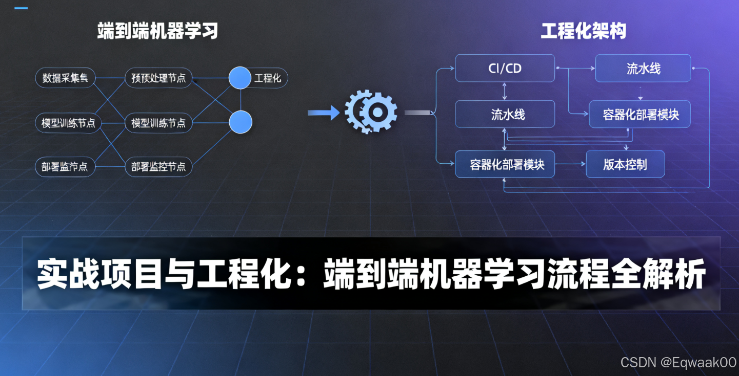
在机器学习项目中，从数据到部署的端到端流程是核心能力。本文将以一个房价预测项目为例，系统讲解完整工程化流程，涵盖数据准备、模型选择、训练调优、部署落地四大环节，并提供可落地的代码方案。

二、数据准备：清洗、特征工程与划分

2.1 数据清洗

2.1.1 缺失值处理

import pandas as pd# 加载数据
data = pd.read_csv('house_prices.csv')# 缺失值统计
missing = data.isnull().sum()
print("缺失值统计:\n", missing[missing > 0])# 策略1：删除缺失列（缺失率>50%）
threshold = 0.5
cols_to_drop = [col for col in data.columns if data[col].isnull().mean() > threshold]
data = data.drop(columns=cols_to_drop)# 策略2：填充数值型缺失值（均值/中位数）
num_cols = data.select_dtypes(include=['int64', 'float64']).columns
for col in num_cols:data[col] = data[col].fillna(data[col].median())# 策略3：填充类别型缺失值（众数）
cat_cols = data.select_dtypes(include=['object']).columns
for col in cat_cols:data[col] = data[col].fillna(data[col].mode()[0])

2.1.2 异常值检测

import numpy as np# 使用IQR方法检测异常值
def detect_outliers(df, column):Q1 = df[column].quantile(0.25)Q3 = df[column].quantile(0.75)IQR = Q3 - Q1lower_bound = Q1 - 1.5 * IQRupper_bound = Q3 + 1.5 * IQRreturn df[(df[column] < lower_bound) | (df[column] > upper_bound)]outliers = detect_outliers(data, 'SalePrice')
print(f"异常值数量: {len(outliers)}")# 处理异常值（删除或替换）
data = data[~data.index.isin(outliers.index)]  # 删除异常值

2.2 特征工程

2.2.1 分箱（Binning）

# 将连续变量分箱（如房价按区间分组）
data['SalePrice_bin'] = pd.cut(data['SalePrice'], bins=[0, 100000, 200000, 300000], labels=['Low', 'Medium', 'High'])

2.2.2 编码（Encoding）

from sklearn.preprocessing import LabelEncoder, OneHotEncoder# 标签编码（有序类别）
le = LabelEncoder()
data['OverallQual_encoded'] = le.fit_transform(data['OverallQual'])# 独热编码（无序类别）
ohe = OneHotEncoder(sparse=False)
cat_cols = ['MSZoning', 'Street']
ohe_data = ohe.fit_transform(data[cat_cols])
ohe_df = pd.DataFrame(ohe_data, columns=ohe.get_feature_names_out(cat_cols))
data = pd.concat([data, ohe_df], axis=1)

2.3 数据划分

from sklearn.model_selection import train_test_split# 划分训练集、验证集、测试集（60-20-20）
X = data.drop('SalePrice', axis=1)
y = data['SalePrice']X_train, X_temp, y_train, y_temp = train_test_split(X, y, test_size=0.4, random_state=42)
X_val, X_test, y_val, y_test = train_test_split(X_temp, y_temp, test_size=0.5, random_state=42)print(f"训练集: {X_train.shape}, 验证集: {X_val.shape}, 测试集: {X_test.shape}")

三、模型选择：分类与回归算法

3.1 任务类型判断

任务类型	目标变量类型	示例算法
分类	离散值（如类别）	逻辑回归、随机森林、梯度提升
回归	连续值（如房价）	线性回归、决策树、神经网络

3.2 算法选择指南

3.2.1 回归任务示例（房价预测）

from sklearn.linear_model import LinearRegression
from sklearn.ensemble import RandomForestRegressor
from xgboost import XGBRegressor# 初始化模型
models = {'LinearRegression': LinearRegression(),'RandomForest': RandomForestRegressor(n_estimators=100, random_state=42),'XGBoost': XGBRegressor(n_estimators=100, learning_rate=0.1)
}

3.2.2 分类任务示例（客户流失预测）

from sklearn.linear_model import LogisticRegression
from sklearn.ensemble import GradientBoostingClassifiermodels = {'LogisticRegression': LogisticRegression(max_iter=1000),'GradientBoosting': GradientBoostingClassifier(n_estimators=100)
}

四、训练与调优：交叉验证与Early Stopping

4.1 交叉验证

from sklearn.model_selection import cross_val_score# 5折交叉验证评估模型
for name, model in models.items():scores = cross_val_score(model, X_train, y_train, cv=5, scoring='neg_mean_squared_error')rmse = np.sqrt(-scores.mean())print(f"{name} RMSE: {rmse:.2f}")

4.2 超参数调优

from sklearn.model_selection import GridSearchCV# 随机森林参数网格
param_grid = {'n_estimators': [50, 100, 200],'max_depth': [None, 10, 20],'min_samples_split': [2, 5]
}# 网格搜索
grid_search = GridSearchCV(RandomForestRegressor(), param_grid, cv=5, scoring='neg_mean_squared_error')
grid_search.fit(X_train, y_train)print("最佳参数:", grid_search.best_params_)

4.3 Early Stopping（深度学习示例）

from tensorflow.keras.models import Sequential
from tensorflow.keras.layers import Dense
from tensorflow.keras.callbacks import EarlyStopping# 构建模型
model = Sequential([Dense(64, activation='relu', input_shape=(X_train.shape[1],)),Dense(32, activation='relu'),Dense(1)
])# 编译
model.compile(optimizer='adam', loss='mse')# Early Stopping
early_stop = EarlyStopping(monitor='val_loss', patience=10, restore_best_weights=True)# 训练
history = model.fit(X_train, y_train,validation_data=(X_val, y_val),epochs=100,batch_size=32,callbacks=[early_stop]
)

五、部署落地：序列化与API封装

5.1 模型序列化

5.1.1 Pickle保存

import pickle# 保存模型
with open('random_forest_model.pkl', 'wb') as f:pickle.dump(grid_search.best_estimator_, f)# 加载模型
with open('random_forest_model.pkl', 'rb') as f:loaded_model = pickle.load(f)

5.1.2 ONNX格式（跨平台）

from skl2onnx import convert_sklearn
from skl2onnx.common.data_types import FloatTensorType# 转换模型为ONNX
initial_type = [('float_input', FloatTensorType([None, X_train.shape[1]]))]
onnx_model = convert_sklearn(grid_search.best_estimator_, initial_types=initial_type)# 保存
with open("model.onnx", "wb") as f:f.write(onnx_model.SerializeToString())

5.2 Flask API封装

from flask import Flask, request, jsonify
import pickle
import numpy as npapp = Flask(__name__)# 加载模型
with open('random_forest_model.pkl', 'rb') as f:model = pickle.load(f)@app.route('/predict', methods=['POST'])
def predict():# 获取输入数据data = request.get_json()features = np.array(data['features']).reshape(1, -1)# 预测prediction = model.predict(features)return jsonify({'prediction': prediction.tolist()})if __name__ == '__main__':app.run(host='0.0.0.0', port=5000)

5.3 部署测试

# 启动API
python app.py# 发送测试请求
curl -X POST http://localhost:5000/predict \-H "Content-Type: application/json" \-d '{"features": [0.1, 0.5, 1200, 3, ...]}'

六、完整项目流程图

graph TDA[数据准备] --> B[模型选择]B --> C[训练与调优]C --> D[部署落地]A --> A1[清洗] --> A2[特征工程] --> A3[划分]B --> B1[分类] --> B2[回归]C --> C1[交叉验证] --> C2[超参数调优] --> C3[Early Stopping]D --> D1[序列化] --> D2[API封装]