当前位置：首页 > news >正文

【Block总结】LAGA，大核分组注意力门，实现特征融合|即插即用

news 2025/9/30 10:33:46

论文信息

标题：EMCAD: Efficient Multi-scale Convolutional Attention Decoding for Medical Image Segmentation（EMCAD：用于医学图像分割的高效多尺度卷积注意力解码器）
作者：Md Mostafijur Rahman, Mustafa Munir, Radu Marculescu
论文链接：https://arxiv.org/pdf/2405.06880
核心问题：现有的医学图像分割模型，尤其是结合了注意力机制的解码器，往往计算成本高昂（参数量大、FLOPs高），难以在计算资源受限的场景（如边缘设备、实时诊断）中部署。
核心贡献：提出了一种名为 EMCAD 的新型高效解码器，旨在同时优化分割性能和计算效率。该解码器可以与各种分层视觉编码器（如CNN或Transformer）配合使用。

创新点

论文提出了三个主要的创新模块，共同构成了高效的EMCAD解码器：

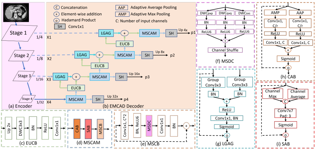
高效的多尺度卷积注意力模块 (MSCAM)：该模块使用 多尺度深度可分离卷积 (Depth-wise Convolution) 来增强特征图，能够有效捕捉多尺度显著特征，同时通过通道注意力和空间注意力机制来聚焦关键区域。深度可分离卷积的使用是其高效的关键。
大核分组注意力门 (LGAG)：这是一种新颖的特征融合机制。与传统的注意力门（如Attention U-Net中使用的1x1卷积）不同，LGAG在处理门控信号和输入特征时，采用了3x3的大核分组卷积。这使得模型能在更大的局部上下文中捕捉显著特征，且计算开销更低。
高效的上卷积块(EUCB)：用于上采样特征图。它使用3x3深度可分离卷积替代了标准的3x3卷积，显著降低了上采样过程中的计算成本。

方法

EMCAD的整体架构是一个级联的全卷积注意力解码器，其工作流程如下：

输入：接收来自预训练分层视觉编码器（如PVTv2）的四个阶段（X1, X2, X3, X4）的多尺度特征图。
特征精炼：每个阶段的特征图首先通过一个 MSCAM 模块进行精炼，该模块依次应用通道注意力（CAB）、空间注意力（SAB）和多尺度卷积块（MSCB）。
中间输出：精炼后的每个阶段特征图都会通过一个**分割头 **(SH) 生成一个中间分割图（p1, p2, p3, p4）。
上采样与融合：
- 从最深层（X4）开始，精炼后的特征图通过 EUCB 进行上采样。
- 上采样后的特征图与来自编码器对应层的跳跃连接（Skip Connection）特征图一起送入 LGAG 模块。
- LGAG利用高层特征作为门控信号，对跳跃连接的特征进行加权，然后与上采样特征相加，实现高效的特征融合。
级联传递：融合后的特征图作为下一级的输入，重复步骤2-4，直至生成最终的高分辨率特征图。
最终输出与损失：论文将最后一个阶段（p4）的分割图作为最终输出。在训练时，采用多阶段损失策略，不仅计算最终输出的损失，还计算所有中间分割图（p1-p4）以及它们的加和的损失，以提供更丰富的监督信号。

在这里插入图片描述

LGAG（Large-kernel Grouped Attention Gate）模块详解

LGAG 是 EMCAD 解码器中用于高效融合上采样特征与跳跃连接（skip connection）特征的关键模块。其设计目标是在保留显著区域信息的同时，显著降低计算开销，特别适用于医学图像分割中对局部上下文敏感的场景。
在这里插入图片描述

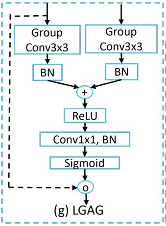
1. 设计动机

传统注意力门（如 Attention U-Net 中的 AG）通常使用 1×1 卷积来处理门控信号（gating signal）和输入特征，这种方式感受野有限，难以捕捉局部空间上下文信息。

LGAG 的创新在于：

使用 3×3 大核卷积
引入 分组卷积（Grouped Convolution）

这使得 LGAG 能在更大的局部感受野中建模空间依赖关系，同时通过分组策略大幅降低参数量和计算量。

2. 模块结构与计算流程

LGAG 接收两个输入：

g：来自高层（上采样路径）的门控信号（gating signal）
x：来自编码器对应层的跳跃连接特征

其计算分为以下几步（对应论文公式 1 和 2）：

步骤 1：分别对 g 和 x 进行 3×3 分组卷积

对门控信号 g：应用分组卷积 $GC_g(g)$
对跳跃特征 x：应用分组卷积 $GC_x(x)$

步骤 2：批归一化（BN）与融合

对 $GC_x(x)$ 先做 BN
将 $GC_g(g)$ 与 $BN(GC_x(x))$ 逐元素相加
对相加结果再做 BN，并通过 ReLU 激活

该过程定义为：
$q_{att}(g, x) = \text{ReLU}\left( \text{BN}\left( GC_g(g) + \text{BN}(GC_x(x)) \right) \right)$

步骤 3：生成注意力权重

对 $q_{att}(g, x)$ 应用 1×1 卷积 + BN，将其压缩为单通道特征图
通过 Sigmoid 激活函数生成注意力权重 $α∈[0,1]\alpha \in [0,1]$

步骤 4：加权输出

将注意力权重 $α\alpha$ 与原始输入特征 x 进行逐元素相乘（Hadamard product）
得到最终的门控输出：

$\text{LGAG}(g, x) = x \circledast \sigma\left( \text{BN}(C(q_{att}(g, x))) \right)$

其中：

$C(⋅)C(\cdot)$ 表示 1×1 卷积
$σ(⋅)\sigma(\cdot)$ 为 Sigmoid 函数
$⊛\circledast$ 表示逐元素相乘

3. 关键优势

特性	说明
大感受野	3×3 卷积相比 1×1 能捕获更大局部上下文，有助于精确定位医学结构边界
计算高效	分组卷积显著减少参数量和 FLOPs（见补充材料 Table 8：相比传统 AG，LGAG 参数减少 82.6%~91.2%）
可扩展性强	在通道数增加时（如 B2 模型），LGAG 的效率优势更加明显
性能提升	在 Synapse 数据集上，使用 LGAG 比传统 AG 提升 DICE 分数（B0: 81.97 vs 81.74；B2: 83.63 vs 83.51）

代码

import torch
import torch.nn as nn
from timm.models.helpers import named_apply
from functools import partial
from timm.models.layers import trunc_normal_tf_# Other types of layers can go here (e.g., nn.Linear, etc.)
def _init_weights(module, name, scheme=''):if isinstance(module, nn.Conv2d) or isinstance(module, nn.Conv3d):if scheme == 'normal':nn.init.normal_(module.weight, std=.02)if module.bias is not None:nn.init.zeros_(module.bias)elif scheme == 'trunc_normal':trunc_normal_tf_(module.weight, std=.02)if module.bias is not None:nn.init.zeros_(module.bias)elif scheme == 'xavier_normal':nn.init.xavier_normal_(module.weight)if module.bias is not None:nn.init.zeros_(module.bias)elif scheme == 'kaiming_normal':nn.init.kaiming_normal_(module.weight, mode='fan_out', nonlinearity='relu')if module.bias is not None:nn.init.zeros_(module.bias)else:# efficientnet likefan_out = module.kernel_size[0] * module.kernel_size[1] * module.out_channelsfan_out //= module.groupsnn.init.normal_(module.weight, 0, math.sqrt(2.0 / fan_out))if module.bias is not None:nn.init.zeros_(module.bias)elif isinstance(module, nn.BatchNorm2d) or isinstance(module, nn.BatchNorm3d):nn.init.constant_(module.weight, 1)nn.init.constant_(module.bias, 0)elif isinstance(module, nn.LayerNorm):nn.init.constant_(module.weight, 1)nn.init.constant_(module.bias, 0)def act_layer(act, inplace=False, neg_slope=0.2, n_prelu=1):# activation layeract = act.lower()if act == 'relu':layer = nn.ReLU(inplace)elif act == 'relu6':layer = nn.ReLU6(inplace)elif act == 'leakyrelu':layer = nn.LeakyReLU(neg_slope, inplace)elif act == 'prelu':layer = nn.PReLU(num_parameters=n_prelu, init=neg_slope)elif act == 'gelu':layer = nn.GELU()elif act == 'hswish':layer = nn.Hardswish(inplace)else:raise NotImplementedError('activation layer [%s] is not found' % act)return layerdef channel_shuffle(x, groups):batchsize, num_channels, height, width = x.data.size()channels_per_group = num_channels // groups# reshapex = x.view(batchsize, groups,channels_per_group, height, width)x = torch.transpose(x, 1, 2).contiguous()# flattenx = x.view(batchsize, -1, height, width)return x#   Efficient up-convolution block (EUCB)
class EUCB(nn.Module):def __init__(self, in_channels, out_channels, kernel_size=3, stride=1, activation='relu'):super(EUCB, self).__init__()self.in_channels = in_channelsself.out_channels = out_channelsself.up_dwc = nn.Sequential(nn.Upsample(scale_factor=2),nn.Conv2d(in_channels, in_channels, kernel_size=kernel_size, stride=stride,padding=kernel_size // 2, groups=in_channels, bias=False),nn.BatchNorm2d(in_channels),act_layer(activation, inplace=True))self.pwc = nn.Sequential(nn.Conv2d(in_channels, out_channels, kernel_size=1, stride=1, padding=0, bias=True))self.init_weights('normal')def init_weights(self, scheme=''):named_apply(partial(_init_weights, scheme=scheme), self)def forward(self, x):x = self.up_dwc(x)x = channel_shuffle(x, self.in_channels)x = self.pwc(x)return x#   Large-kernel grouped attention gate (LGAG)
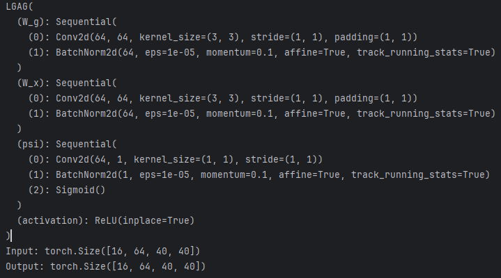
class LGAG(nn.Module):def __init__(self, F_g, F_l, F_int, kernel_size=3, groups=1, activation='relu'):super(LGAG, self).__init__()if kernel_size == 1:groups = 1self.W_g = nn.Sequential(nn.Conv2d(F_g, F_int, kernel_size=kernel_size, stride=1, padding=kernel_size // 2, groups=groups,bias=True),nn.BatchNorm2d(F_int))self.W_x = nn.Sequential(nn.Conv2d(F_l, F_int, kernel_size=kernel_size, stride=1, padding=kernel_size // 2, groups=groups,bias=True),nn.BatchNorm2d(F_int))self.psi = nn.Sequential(nn.Conv2d(F_int, 1, kernel_size=1, stride=1, padding=0, bias=True),nn.BatchNorm2d(1),nn.Sigmoid())self.activation = act_layer(activation, inplace=True)self.init_weights('normal')def init_weights(self, scheme=''):named_apply(partial(_init_weights, scheme=scheme), self)def forward(self, g, x):g1 = self.W_g(g)x1 = self.W_x(x)psi = self.activation(g1 + x1)psi = self.psi(psi)return x * psiif __name__ == "__main__":# 定义输入张量大小（Batch、Channel、Height、Wight）B, C, H, W = 16, 64, 40, 40input_tensor = torch.randn(B, C, H, W)  # 随机生成输入张量input_tensor1 = torch.randn(B, C, H, W)  # 随机生成输入张量dim = C# 创建 ARConv 实例block = LGAG(dim,dim,dim)device = torch.device("cuda" if torch.cuda.is_available() else "cpu")sablock = block.to(device)print(sablock)input_tensor = input_tensor.to(device)input_tensor1 = input_tensor1.to(device)# 执行前向传播output = sablock(input_tensor,input_tensor1)# 打印输入和输出的形状print(f"Input: {input_tensor.shape}")print(f"Output: {output.shape}")

在这里插入图片描述

效果

论文在12个涵盖6种不同医学图像分割任务（息肉、皮肤病变、细胞、乳腺癌、腹部器官、心脏器官）的公共数据集上进行了广泛的实验，结果证明了EMCAD的优越性：

性能领先：提出的 PVT-EMCAD-B2 模型在多个数据集上达到了新的SOTA（State-of-the-Art）性能。例如：
- 在10个二值分割数据集上的平均DICE得分为 91.10%。
- 在Synapse腹部多器官分割数据集上的平均DICE得分为 83.63%。
- 在ACDC心脏分割数据集上的平均DICE得分为 92.12%。
效率极高：EMCAD在取得优异性能的同时，计算成本极低。
- 与强大的基线模型 PVT-CASCADE 相比，EMCAD在Synapse数据集上以 79.4%更少的参数（1.91M vs 9.27M）和 80.3%更少的FLOPs（0.381G vs 1.93G）实现了更高的DICE分数（83.63% vs 82.78%）。
- 其小型版本 PVT-EMCAD-B0 仅需 3.92M参数和 0.84G FLOPs，性能就远超许多现有方法。
通用性强：EMCAD可以无缝集成到不同的分层编码器（如PVTv2-B0, PVTv2-B2）中，并在各种分割任务上均表现出色，证明了其良好的通用性和适应性。