线性代数 | REF / RREF
注:本文为 “线性代数 | REF / RREF” 相关区别与讨论合辑。
英文引文,机翻未校。
中文引文,略作重排。
图片清晰度受引文原图所限。
如有内容异常,请看原文。
Row Echelon Form & Reduced Row Echelon Form
行阶梯形矩阵与简化行阶梯形矩阵
What is Echelon Form?
什么是阶梯形(Echelon Form)?
Echelon form means that the matrix is in one of two states:
阶梯形指矩阵处于以下两种状态之一:
-
Row echelon form.
行阶梯形矩阵 -
Reduced row echelon form.
简化行阶梯形矩阵
This means that the matrix meets the following three requirements:
这意味着该矩阵需满足以下三个条件:
-
The first number in the row (called a leading coefficient) is 1. Note: some authors don’t require that the leading coefficient is a 1; it could be any number. You may want to check with your instructor to see which version of this rule they are adhering to).
每行的第一个非零数(称为首项系数(leading coefficient))为 1。注:部分学者不要求首项系数必须为 1,也可以是任意非零数。建议向授课教师确认其遵循的规则版本。 -
Every leading 1 is to the right of the one above it.
每个首项系数 1 都位于其上方首项系数 1 的右侧。 -
Any non-zero rows are always above rows with all zeros.
所有非零行均位于全零行的上方。
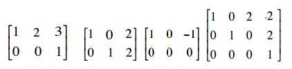
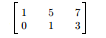
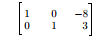
The following examples are of matrices in echelon form:
以下是阶梯形矩阵的示例:
The following examples are not in echelon form:
以下是非阶梯形矩阵的示例:
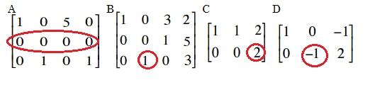
Matrix A does not have all-zero rows below non-zero rows.
矩阵 A 的全零行未位于非零行下方。
Matrix B has a 1 in the 2nd position on the third row. For row echelon form, it needs to be to the right of the leading coefficient above it. In other words, it should be in the fourth position in place of the 3.
矩阵 B 的第三行第 2 列位置为 1,而行阶梯形矩阵要求该首项系数需位于其上方首项系数的右侧,即应在第 4 列(原 3 所在的位置)。
Matrix C has a 2 as a leading coefficient instead of a 1.
矩阵 C 的首项系数(leading coefficient)为 2,而非 1。
Matrix D has a -1 as a leading coefficient instead of a 1.
矩阵 D 的首项系数为 -1,而非 1。
Another way to think of a matrix in echelon form is that the matrix has undergone Gaussian elimination, which is a series of row operations.
从另一个角度理解,阶梯形矩阵是经过高斯消元法(Gaussian elimination)处理后的矩阵,高斯消元法本质是一系列的行变换操作。
Uniqueness and Echelon Forms
阶梯形矩阵的唯一性
The echelon form of a matrix isn’t unique, which means there are infinite answers possible when you perform row reduction. Reduced row echelon form is at the other end of the spectrum; it is unique, which means row-reduction on a matrix will produce the same answer no matter how you perform the same row operations.
矩阵的阶梯形形式不唯一,这意味着对矩阵进行行约简时,可能得到[无穷多(infinite)个不同的结果。而简化行阶梯形矩阵则完全相反,它具有唯一性——无论采用何种行变换顺序对矩阵进行行约简,最终得到的简化行阶梯形矩阵始终相同。
What is Row Echelon Form?
什么是行阶梯形矩阵(Row Echelon Form)?
A matrix is in row echelon form if it meets the following requirements:
满足以下条件的矩阵即为行阶梯形矩阵:
-
The first non-zero number from the left (the “leading coefficient“) is always to the right of the first non-zero number in the row above.
每行从左起的第一个非零数(即“首项系数(leading coefficient)”),始终位于其上方一行首项系数的右侧。 -
Rows consisting of all zeros are at the bottom of the matrix.
所有全零行均位于矩阵的底部。
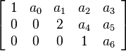
Row echelon form. “a” can represent any number.
行阶梯形矩阵。其中“a”可表示任意数值。
Technically, the leading coefficient can be any number. However, the majority of Linear Algebra textbooks do state that the leading coefficient must be the number 1. To add to the confusion, some definitions of row echelon form state that there must be zeros both above and below the leading coefficient. It’s therefore best to follow the definition given in the textbook you’re following (or the one given to you by your professor). If you’re unsure (i.e. it’s Sunday, your homework is due and you can’t get hold of your professor), it safest to use 1 as the leading coefficient in each row.
从技术层面而言,首项系数可以是任意非零数。但大多数《线性代数》教材明确要求首项系数必须为 1。更易混淆的是,部分行阶梯形矩阵的定义还要求首项系数的“上方和下方均为零”。因此,最佳做法是遵循所使用教材(或授课教师)给出的定义。若无法确认(例如周日需提交作业却联系不上教师),最稳妥的方式是将每行首项系数均设为 1。
If the leading coefficient in each row is the only non-zero number in that column, the matrix is said to be in reduced row echelon form.
若每行首项系数是其所在列中唯一的非零数,则该矩阵为简化行阶梯形矩阵。
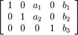
A 3×5 matrix in reduced row echelon form.
一个 3×5 的简化行阶梯形矩阵。
Row echelon forms are commonly encountered in linear algebra, when you’ll sometimes be asked to convert a matrix into this form. The row echelon form can help you to see what a matrix represents and is also an important step to solving systems of linear equations.
行阶梯形矩阵是线性代数中的常见形式,学习过程中常会遇到“将矩阵化为行阶梯形”的任务。行阶梯形矩阵不仅能帮助理解矩阵的本质含义,也是求解线性方程组的重要步骤。
Online Row Echelon Form Calculator
在线行阶梯形矩阵计算器
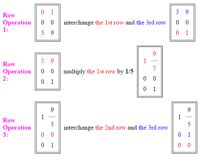
This online calculator will convert any matrix, and provides the row operations that get you from step to step. The following image (from the Old Dominion University Calculator shows how the matrix [01, 00, 59] is reduced to row echelon form with two simple row operations:
此在线计算器可将任意矩阵化为行阶梯形,并提供每一步的行变换过程。下图(来自老道明大学计算器)展示了如何通过两次简单的行变换,将矩阵 [01, 00, 59] 化为行阶梯形:
What is Reduced Row Echelon Form?
什么是简化行阶梯形矩阵(Reduced Row Echelon Form)?
Reduced row echelon form is a type of matrix used to solve systems of linear equations. Reduced row echelon form has four requirements:
简化行阶梯形矩阵是一种用于求解线性方程组(linear equations)的矩阵形式,需满足以下四个条件:
-
The first non-zero number in the first row (the leading entry) is the number 1.
第一行的第一个非零数(首项元素(leading entry))为 1。 -
The second row also starts with the number 1, which is further to the right than the leading entry in the first row. For every subsequent row, the number 1 must be further to the right.
第二行的首项元素也为 1,且位于第一行首项元素的右侧;后续每行的首项元素 1 均需位于前一行首项元素的右侧。 -
The leading entry in each row must be the only non-zero number in its column.
每行的首项元素必须是其所在列中唯一的非零数。 -
Any zero rows are placed at the bottom of the matrix.
所有全零行均位于矩阵的底部。
A 3×5 matrix in reduced row echelon form.
一个 3×5 的简化行阶梯形矩阵。
Transformation of a Matrix to Reduced Row Echelon Form
矩阵化为简化行阶梯形的方法
Any matrix can be transformed to reduced row echelon form, using a technique called Gaussian elimination. This is particularly useful for solving systems of linear equations. Most graphing calculators (like the TI-83) have a rref function which will transform a matrix into a reduced row echelon form. See: This article on the Colorado State University website for instructions on using the TI-89 and TI-83 to calculate reduced row echelon form.
任意矩阵都可通过“高斯消元法(Gaussian elimination)”转化(transformed)为简化行阶梯形,该方法在求解线性方程组时尤为实用。大多数图形计算器(如 TI-83)都配备“rref”函数,可直接将矩阵化为简化行阶梯形。
This online calculator on the Old Dominion University website transforms a matrix that you input to reduced row echelon form.
老道明大学网站的此在线计算器可将输入的任意矩阵化为简化行阶梯形。
Calculation by hand requires knowledge of elementary row operations, which are:
手动计算时,需掌握以下三种初等行变换(elementary row operations):
-
Interchange one row with another.
交换任意两行 -
Multiply one row by a non-zero constant.
用一个非零常数乘以某一行 -
Replace one row with: one row, plus a constant, times another row.
将某一行替换为“该行加上另一行与某一常数的乘积”
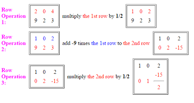
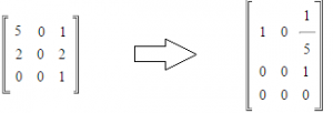
In addition, it isn’t enough just to know the rules, you have to be able to look at the matrix and make a logical decision about which rule you’re going to use and when. You’re trying to get the matrix into reduced row echelon form, so you’ll also need to refer to the four requirements at the beginning of this article. If you have to convert a matrix to reduced row echelon form by hand, it’s a good idea to use one of the calculators above to check your work. In fact, if you use the ODU online calculator, it will even provide the row operations for you. The image below is the calculator’s conversion of the matrix [204,923]:
此外,仅掌握规则是不够的,还需根据矩阵的具体结构,合理判断何时使用何种变换。由于目标是化为简化行阶梯形,过程中需时刻对照本文开头列出的四个条件。若需手动计算,建议使用上述计算器验证结果;事实上,使用老道明大学在线计算器还可直接获取每一步的行变换过程。下图为该计算器将矩阵 [204, 923] 化为简化行阶梯形的结果:
What is Gaussian Elimination?
什么是高斯消元法(Gaussian Elimination)?
Gaussian elimination is a way to find a solution to a system of linear equations. The basic idea is that you perform a mathematical operation on a row and continue until only one variable is left. For example, some possible row operations are:
高斯消元法是求解线性方程组的一种方法,核心思想是通过对矩阵的行进行数学运算,逐步消元,最终使每行仅保留一个变量(variable)。常见的行变换示例包括:
-
Interchange any two rows
交换任意两行 -
Add two rows together.
将两行相加 -
Multiply one row by a non-zero constant (i.e. 1/3, -1, 5)You can also perform more than one row operation at a time. For example, multiply one row by a constant and then add the result to the other row.
你也可以同时执行多个行变换操作。例如,先将某一行乘以一个常数,再将结果与另一行相加。
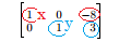
Following this, the goal is to end up with a matrix in reduced row echelon form where the leading coefficient, a 1, in each row is to the right of the leading coefficient in the row above it. In other words, you need to get a 1 in the upper left corner of the matrix. The next row should have a 0 in position 1 and a 1 in position 2. This gives you the solution to the system of linear equations.
通过这些操作,最终目标是将矩阵化为简化行阶梯形——每行的首项系数(值为 1)需位于其上方行首项系数的右侧。具体来说,需先在矩阵左上角得到一个 1;下一行则需在第 1 列位置为 0,第 2 列位置为 1。此时,即可直接读出线性方程组的解。
Gaussian Elimination Example
高斯消元法示例
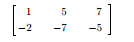
Solve the following system of linear equations using Gaussian elimination:
使用高斯消元法求解以下线性方程组:
-
x+5y=7x + 5y = 7x+5y=7
-
−2x−7y=−5-2x - 7y = -5−2x−7y=−5
Step 1: Convert the equation into coefficient matrix form. In other words, just take the coefficient for the numbers and forget the variables for now:
步骤 1:将方程组转化为系数矩阵形式。即仅保留未知数的系数,暂时忽略变量本身:
Step 2: Turn the numbers in the bottom row into positive by adding 2 times the first row:
步骤 2:将第一行乘以 2 后与第二行相加,使第二行(底行)的第一个元素变为正数:
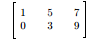
Step 3: Multiply the second row by ( 1/3 ). This gives you your second leading 1:
步骤 3:将第二行乘以 ( 1/3 ),得到第二个首项系数 1:
Step 4: Multiply row 2 by -5, and then add this to row 1:
That’s it!
步骤 4:将第二行乘以 -5 后与第一行相加:
消元完成!
In the first row, you have ( x = -8 ) and in the second row, ( y = 3 ). Note that ( x ) and ( y ) are in the same positions as when you converted the equation in step 1, so all you have to do is read the solution:
此时,第一行对应 ( x = -8 ),第二行对应 ( y = 3 )。需注意,( x ) 和 ( y ) 的位置与步骤 1 中转化系数矩阵时的未知数顺序一致,因此可直接读出方程组的解:
What is the Rank of a Matrix?
什么是矩阵的秩(Rank of a Matrix)?
The rank of a matrix is equal to the number of linearly independent rows. A linearly independent row is one that isn’t a combination of other rows.
矩阵的秩等于矩阵中线性无关(linearly independent)行的数量。线性无关行指无法由其他行通过线性组合得到的行。
The following matrix has two linearly independent rows (1 and 2). However, when the third row is thrown into the mix, you can see that the first row is now equal to the sum of the second and third rows. Therefore, the rank of this particular matrix is 2, as there are only two linearly independent rows.
下图中的矩阵包含 2 个线性无关行(第 1 行和第 2 行)。但加入第 3 行后可见,第 1 行可表示为第 2 行与第 3 行的和,因此该矩阵的秩为 2(仅存在 2 个线性无关行)。
The matrix rank will always be less than the number of non-zero rows or the number of columns in the matrix. If all of the rows in a matrix are linearly independent, the matrix is full row rank. For a square matrix, it is only full row rank if its determinant is non-zero.
矩阵的秩始终小于矩阵的非零行数或列数。若矩阵的所有行均线性无关,则该矩阵具有行满秩(full row rank)。对于方阵(行数等于列数的矩阵),仅当其行列式(determinant)不为零时,才具有行满秩。
Figuring out the rank of a matrix by trying to determine by sight only how many rows or columns are linearly independent can be practically impossible. An easier (and perhaps obvious) way is to convert to row echelon form.
仅通过肉眼观察判断矩阵中线性无关行/列的数量,进而确定秩,在多数情况下难以实现。更简便(且直观)的方法是先将矩阵化为行阶梯形。
How to Find the Matrix Rank
如何求矩阵的秩?
Finding the rank of a matrix is simple if you know how to find the row echelon matrix. To find the rank of any matrix:
只要掌握将矩阵化为行阶梯形的方法,求矩阵的秩就会非常简单。任意矩阵的秩可通过以下步骤求得:
-
Find the row echelon matrix.
将矩阵化为行阶梯形。 -
Count the number of non-zero rows.
统计行阶梯形矩阵中非零行的数量,该数量即为矩阵的秩。
Conversion of a matrix to row echelon form.
矩阵化为行阶梯形的过程。
The above matrix has been converted to row echelon form with two non-zero rows. Therefore, the rank of the matrix is 2.
上述矩阵化为行阶梯形后,包含 2 个非零行,因此该矩阵的秩为 2。
You can also find an excellent conversion tool on the Old Dominion University website.
你也可以使用老道明大学网站上的工具,便捷地将矩阵化为行阶梯形并确定秩。
References
参考文献
Everitt, B. S.; Skrondal, A. (2010), The Cambridge Dictionary of Statistics, Cambridge University Press.
埃弗里特,B. S.;斯克隆达尔,A.(2010),《剑桥统计学词典》,剑桥大学出版社。
Gonick, L. (1993). The Cartoon Guide to Statistics. HarperPerennial.
戈尼克,L.(1993),《统计学漫画指南》,哈珀 perennial 出版社。
Searle, S. (2017). Matrix Algebra Useful for Statistics (Wiley Series in Probability and Statistics) 2nd Edition. Wiley.
塞尔,S.(2017),《统计学实用矩阵代数(威立概率与统计系列)第二版》,威立出版社。
Understanding the Difference Between RREF and REF: Key Concepts and Applications
理解行阶梯形矩阵(REF)与简化行阶梯形矩阵(RREF)的区别:关键概念与应用
Linear algebra might seem like a maze of numbers and equations, but it’s also a world where structure and simplicity reign. If you’ve ever worked with matrices, you know they hold the key to solving complex systems. But simplifying them, two terms often come up—reduced row echelon form (RREF) and row echelon form (REF). At first glance, they might feel interchangeable, yet their differences are crucial.
线性代数看似是由数字和方程构成的迷宫,但它也是一个结构清晰、简洁至上的领域。如果你接触过矩阵,就会知道矩阵是求解复杂方程组的关键。而在对矩阵进行简化时,常会遇到两个术语——简化行阶梯形矩阵(RREF)和行阶梯形矩阵(REF)。初看之下,二者似乎可以互换,但它们之间的差异至关重要。
Picture trying to decode a puzzle where every step matters. RREF is like completing the puzzle perfectly, leaving no ambiguity behind. REF, on the other hand, stops just short of perfection—organized but not fully simplified. Understanding these distinctions doesn’t just make your calculations easier; it sharpens your problem-solving skills in ways you didn’t expect.
不妨想象破解一个每一步都至关重要的谜题:RREF 如同将谜题完美破解,毫无模糊之处;而 REF 则差一步达到完美——虽有条理,但未完全简化。理解这些差异不仅能让计算更轻松,还能以意想不到的方式提升你的解题能力。
So what sets them apart? Let’s jump into how these forms work and why knowing the difference can transform your approach to matrices.
那么,二者的区别究竟是什么?接下来我们将深入探讨这两种矩阵形式的原理,以及了解它们的差异为何能改变你处理矩阵的思路。
Understanding REF (Row Echelon Form)
理解行阶梯形矩阵(REF)
Row Echelon Form (REF) represents a simplified matrix format used to solve linear equations. It’s structured yet less refined compared to RREF, offering partial clarity in computations.
行阶梯形矩阵(REF)是一种用于求解线性方程组的简化矩阵形式。与 RREF 相比,它虽有一定结构,但不够精细,只能为计算提供部分清晰性。
Definition And Characteristics
定义与性质
REF is a matrix form where each non-zero row has more leading zeros than the previous row. The leading entry of every row lies in a column to the right of the leading entry above it. Rows containing all zeros are positioned at the bottom.
行阶梯形矩阵(REF)具有以下特征:每个非零行的前导零个数多于前一行;每行的前导元素(主元)所在列位于上一行前导元素所在列的右侧;全零行(若存在)均位于矩阵底部。
For example, consider this 3×33 \times 33×3 matrix:
例如,以下是一个 3×33 \times 33×3 矩阵:
[123045006]\begin{bmatrix} 1 & 2 & 3 \\ 0 & 4 & 5 \\ 0 & 0 & 6 \end{bmatrix} 100240356
The structure satisfies REF rules but isn’t fully reduced as it allows non-zero entries above pivot points.
该矩阵的结构符合 REF 的规则,但并未完全简化,因为其主元上方允许存在非零元素。
Steps To Achieve REF
化为行阶梯形矩阵(REF)的步骤
-
Identify Pivot Elements: Begin with the leftmost column and locate the first non-zero element.
确定主元:从最左侧列开始,找到该列的第一个非零元素。 -
Reorder Rows If Necessary: Place rows with pivot elements higher up if they’re not already.
必要时交换行:若主元所在行不在上方,则将其移至更靠上的位置。 -
Eliminate Below Pivots: Use elementary row operations to zero out entries below each pivot point.
消去主元下方元素:通过初等行变换,将每个主元下方的元素化为 000。 -
Repeat for Next Columns: Progress rightward, repeating these steps until achieving REF.
对后续列重复操作:向右移动,重复上述步骤,直至将矩阵化为 REF。
When working on larger matrices like a system of equations with four variables, these steps help streamline calculations without overcomplicating them early in simplification.
在处理较大矩阵(如含 444 个变量的方程组对应的矩阵)时,这些步骤能在简化初期避免计算过于复杂,从而提高计算效率。
Applications Of REF
行阶梯形矩阵(REF)的应用
REF simplifies solving linear systems via back-substitution when determining variable values quickly becomes essential. It’s commonly applied in Gaussian elimination methods and offers an intermediate step toward finding determinants or inverses for square matrices.
当需要快速确定变量值时,REF 可通过回代法简化线性方程组的求解过程。它常用于高斯消元法,同时也是求方阵的行列式或逆矩阵的中间步骤。
In practical terms, engineers use REF when analyzing electrical circuits or optimizing resource allocation models due its computational efficiency before full reduction to RREF. Students often encounter this form as their initial approach towards understanding matrix transformations and vector spaces within linear algebra courses.
在实际应用中,由于在完全化为 RREF 之前,REF 具有更高的计算效率,工程师会在电路分析或资源分配模型优化中使用它。在线性代数课程中,学生也常会先接触 REF,以此作为理解矩阵变换和向量空间的入门方式。
Understanding RREF (Reduced Row Echelon Form)
理解简化行阶梯形矩阵(RREF)
RREF represents a fully simplified matrix form in linear algebra, offering precision and clarity unmatched by other forms. It’s an essential tool for solving systems of linear equations efficiently.
在线性代数(linear algebra)中,简化行阶梯形矩阵(RREF)是一种完全简化的矩阵形式,其精度和清晰度是其他矩阵形式无法比拟的,也是高效求解线性方程组的重要工具。
Definition And Characteristics
定义与性质
Reduced row echelon form is characterized by strict rules ensuring uniformity. Each leading entry in a non-zero row equals 111 and appears to the right of any leading entries above it. All entries below and above a leading 111 are zeroes, creating distinct pivot columns. Rows containing only zeroes, if present, are positioned at the bottom.
简化行阶梯形矩阵(RREF)具有严格的规则,以确保其一致性:非零行的前导元素(主元)均为 111,且每个主元所在列位于上一行主元所在列的右侧;主元(即前导 111)的上下元素均为 000,形成明确的主元列;全零行(若存在)均位于矩阵底部。
Unlike REF, RREF eliminates ambiguity entirely by enforcing these additional conditions beyond merely arranging rows in order of pivots. For example:
与 REF 不同,RREF 除了要求按主元顺序排列行之外,还通过上述额外条件完全消除了模糊性。例如:
A matrix in REF:
一个行阶梯形矩阵(REF)如下:
[123045006]\begin{bmatrix} 1 & 2 & 3 \\ 0 & 4 & 5 \\ 0 & 0 & 6 \end{bmatrix} 100240356
Its equivalent RREF:
其对应的简化行阶梯形矩阵(RREF)如下:
[10−7201−54001]\begin{bmatrix} 1 & 0 & -\frac{7}{2} \\ 0 & 1 & -\frac{5}{4} \\ 0 & 0 & 1 \end{bmatrix} 100010−27−451
Notice how every column with a pivot has zeros elsewhere and how each pivot stands alone as “111”.
可见,每个主元所在列的其他元素均为 000,且每个主元均为独立的“111”。
Steps To Achieve RREF
化为简化行阶梯形矩阵(RREF)的步骤
Achieving RREF requires systematic operations that refine an initial matrix into its final form:
将矩阵化为 RREF 需要通过系统性的操作逐步优化,具体步骤如下:
-
Identify Pivots: Locate the first non-zero element in each row from left to right.
确定主元:从左到右,找到每行的第一个非零元素。 -
Normalize Rows: Scale rows so that each pivot becomes exactly “111”.
行标准化:对行进行缩放,使每个主元恰好为“111”。 -
Eliminate Non-Zero Entries: Use row operations to ensure all other elements in the pivot’s column become zero.
消去非零元素:通过行变换,确保主元所在列的其他所有元素均化为 000。 -
Reorder Rows If Necessary: Arrange rows such that lower rows don’t contain pivots further left than those above them.
必要时交换行:调整行的顺序,确保下方行的主元不会位于上方行主元的左侧。
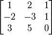
For instance, starting with:
例如,从以下矩阵开始:
[2−4−63−9−126−12−18]\begin{bmatrix} 2 & -4 & -6 \\ 3 & -9 & -12 \\ 6 & -12 & -18 \end{bmatrix} 236−4−9−12−6−12−18
After applying steps sequentially:
依次应用上述步骤后:
[1−2−3033000]\begin{bmatrix} 1 & -2 & -3 \\ 0 & 3 & 3 \\ 0 & 0 & 0 \end{bmatrix} 100−230−330
Even small errors here can lead to incorrect results!
此处即使出现微小错误,也可能导致结果出错!
Key Differences Between REF And RREF
行阶梯形矩阵(REF)与简化行阶梯形矩阵(RREF)的关键区别
Understanding the distinctions between row echelon form (REF) and reduced row echelon form (RREF) enhances your ability to work with matrices effectively. While both are systematic matrix forms, their structures and applications differ significantly.
理解行阶梯形矩阵(REF)与简化行阶梯形矩阵(RREF)的区别,能提升你高效处理矩阵的能力。尽管二者均为系统性的矩阵形式,但它们的结构和应用存在显著差异。
Structure And Form
结构与形式
The structure of REF involves rows where each pivot element appears further to the right than in the preceding row. Rows consisting entirely of zeros align at the bottom, ensuring a triangular arrangement. In contrast, RREF requires stricter conditions: every leading entry is 111, all entries above and below these leading ones are zeroes, and pivots proceed diagonally from left to right without ambiguity.
REF 的结构要求:每个主元所在列位于前一行主元所在列的右侧,全零行位于底部,整体呈三角排列。相比之下,RREF 的要求更为严格:每个前导元素(主元)均为 111,主元的上下元素均为 000,且主元从左到右呈对角线方向排列,无任何模糊性。
For example, in REF:
例如,行阶梯形矩阵(REF)如下:
[234056007]\begin{bmatrix} 2 & 3 & 4 \\ 0 & 5 & 6 \\ 0 & 0 & 7 \end{bmatrix} 200350467
In RREF:
简化行阶梯形矩阵(RREF)如下:
[10x01y00z]\begin{bmatrix} 1 & 0 & x \\ 0 & 1 & y \\ 0 & 0 & z \end{bmatrix} 100010xyz
This distinction makes RREF more precise but also more computationally intensive to achieve.
这种差异使得 RREF 的精度更高,但化为 RREF 的计算量也更大。
Computational Process
计算过程
Achieving REF relies on Gaussian elimination steps like row swapping, multiplying rows by non-zero scalars, and adding/subtracting multiples of rows. The process stops once pivot elements meet the triangular pattern criteria. But achieving RREF extends this by normalizing each pivot to one and eliminating non-zero entries above pivots through additional operations.
化为 REF 依赖于高斯消元的步骤,包括交换行、将行乘以非零标量、将一行的倍数与另一行相加或相减。当主元满足三角排列条件时,该过程即可停止。而化为 RREF 则需要在 REF 的基础上进一步操作:将每个主元标准化为 111,并通过额外的行变换消去主元上方的非零元素。
Due to its complexity, transitioning from REF to RREF often consumes more time in large matrices. For instance, when solving a system with four equations and four unknowns, converting directly into RREF may involve extra calculations compared to stopping at REF followed by back-substitution.
由于计算更复杂,在处理大型矩阵时,从 REF 进一步化为 RREF 通常需要更多时间。例如,在求解含 444 个方程和 444 个未知数的方程组时,直接将矩阵化为 RREF 所需的计算量,会比先化为 REF 再通过回代法求解更多。
Use Cases And Practical Implications
应用场景与实际意义
Engineers leverage REF for initial simplifications during circuit analysis or resource allocation optimization as it allows quick identification of dependent variables. Students frequently use it while learning linear algebra because it’s less intricate than working directly with RREF.
工程师在电路分析或资源分配优化中,会利用 REF 进行初步简化,因为它能快速识别因变量。在学习线性代数时,学生也常使用 REF,因为它比直接处理 RREF 更简单。
RREF, however, shines in scenarios demanding precision. It’s indispensable in computer algorithms for data science (e.g., linear regression, principal component analysis) where exact solutions prevent errors in model predictions. Additionally, RREF simplifies verifying the uniqueness of solutions for linear systems—if the RREF of an augmented matrix has a row like [000∣c]\begin{bmatrix} 0 & 0 & 0 \mid c \end{bmatrix}[000∣c] (where c≠0c \neq 0c=0), the system is inconsistent and has no solution.
然而,在对精度要求较高的场景中,RREF 的优势更为明显。在数据科学的计算机算法(如线性回归、主成分分析)中,RREF 不可或缺,因为精确的解能避免模型预测出现误差。此外,RREF 还能简化线性方程组解的唯一性验证:若增广矩阵的 RREF 中出现形如 [000∣c]\begin{bmatrix} 0 & 0 & 0 \mid c \end{bmatrix}[000∣c](其中 c≠0c \neq 0c=0)的行,则该方程组无解(不相容)。
Why Understanding These Differences Matters
为何理解这些差异至关重要
Grasping the distinctions between RREF and REF enhances your ability to solve linear algebra problems efficiently. When you understand how each form structures matrices, you can choose the most effective method for specific tasks. For example, if you’re solving a system of equations quickly, REF simplifies calculations using back-substitution. But, in scenarios requiring exact solutions or verifying uniqueness—such as computer algorithms in data science—RREF offers precision.
掌握 RREF 与 REF 的差异,能提升你高效求解线性代数问题的能力。理解每种矩阵形式的结构后,你可以为特定任务选择最有效的方法。例如,若需快速求解方程组,REF 可通过回代法简化计算;而在需要精确解或验证解的唯一性的场景(如数据科学中的计算机算法)中,RREF 能提供更高的精度。
Mastering these differences benefits both academic and professional pursuits. In engineering applications like circuit analysis, recognizing when to stop at REF versus continuing to RREF saves time without compromising results. Similarly, students tackling Gaussian elimination develop stronger problem-solving skills by evaluating which matrix form aids their goals better.
掌握这些差异对学术和职业发展都有帮助。在电路分析等工程应用中,判断何时只需将矩阵化为 REF、何时需进一步化为 RREF,既能节省时间,又不会影响结果准确性。同样,在学习高斯消元法时,学生通过判断哪种矩阵形式更符合解题目标,能培养更强的解题能力。
Ignoring these differences risks errors in computations and misinterpretation of results. Picture relying on REF when a fully simplified solution is needed; this could lead to incomplete or ambiguous answers, especially in contexts demanding high accuracy like econometrics or machine learning models.
忽视这些差异可能导致计算错误和结果解读偏差。例如,在需要完全简化的解的场景中,若仍依赖 REF,可能会得到不完整或模糊的答案——尤其是在计量经济学或机器学习模型等对精度要求极高的领域。
Recognizing why RREF requires stricter conditions also deepens your understanding of linear transformations’ intricacies. This knowledge sharpens analytical capabilities across disciplines—from physics to computational biology—where matrices model complex systems effectively.
理解 RREF 为何需要更严格的条件,还能加深你对线性变换复杂性的认识。这种知识能提升跨学科的分析能力,在物理学、计算生物学等领域(矩阵是这些领域中建模复杂系统的有效工具)都能发挥作用。
Conclusion
结论
Grasping the differences between REF and RREF equips you with a deeper understanding of matrix transformations, enabling better decision-making in solving linear systems. Whether you’re simplifying equations for quick results or seeking precision in high-stakes applications, knowing when to use each form is invaluable.
掌握 REF 与 RREF 的差异,能让你更深入地理解矩阵变换,从而在求解线性方程组时做出更合理的决策。无论你是为快速得到结果而简化方程,还是在高风险应用中追求精度,知道何时使用哪种矩阵形式都具有重要价值。
By mastering these concepts, you enhance your problem-solving skills and build a foundation for tackling complex challenges across various fields. Understanding REF and RREF isn’t just about completing calculations; it’s about unlocking efficiency and accuracy in your mathematical approach.
掌握这些概念,能提升你的解题能力,并为应对各领域的复杂挑战奠定基础。理解 REF 和 RREF 不仅仅是为了完成计算,更是为了在数学方法中实现高效与精准的统一。
Differences Between Row Echelon and Reduced Row Echelon
行最简形与简化行最简形之间的差异
Let
令
A=[13−62512−247915−306]A = \begin{bmatrix} 1 & 3 & -6 & 2 \\ 5 & 12 & -24 & 7 \\ 9 & 15 & -30 & 6 \end{bmatrix}A=15931215−6−24−30276
RREF(A)=[100−101−2−10000]\text{RREF}(A) = \begin{bmatrix} 1 & 0 & 0 & -1 \\ 0 & 1 & -2 & -1 \\ 0 & 0 & 0 & 0 \end{bmatrix}RREF(A)=1000100−20−1−10
REF(A)=[13−6201−210000]\text{REF}(A) = \begin{bmatrix} 1 & 3 & -6 & 2 \\ 0 & 1 & -2 & 1 \\ 0 & 0 & 0 & 0 \end{bmatrix}REF(A)=100310−6−20210
Now, provided this information, it can be found that the basis for the nullspace of AAA using the RREF(A)\text{RREF}(A)RREF(A) is:
基于上述信息,可以得出利用 RREF(A)\text{RREF}(A)RREF(A) 求得的 AAA 的零空间的基为:
([0210],[1−101])\left( \begin{bmatrix} 0 \\ 2 \\ 1 \\ 0 \end{bmatrix}, \begin{bmatrix} 1 \\ -1 \\ 0 \\ 1 \end{bmatrix} \right)0210,1−101
Using the REF(A)\text{REF}(A)REF(A) the “basis” for the nullspace is:
利用 REF(A)\text{REF}(A)REF(A) 求得的零空间的“基”为:
([6210],[−2−101])\left( \begin{bmatrix} 6 \\ 2 \\ 1 \\ 0 \end{bmatrix}, \begin{bmatrix} -2 \\ -1 \\ 0 \\ 1 \end{bmatrix} \right)6210,−2−101
Is the “basis” that I provided for the REF(A)\text{REF}(A)REF(A) actually a basis? How does the REF\text{REF}REF and RREF\text{RREF}RREF of a matrix differ?
我所给出的 REF(A)\text{REF}(A)REF(A) 的“基”真的是一个基吗?矩阵的 REF\text{REF}REF 和 RREF\text{RREF}RREF 有何不同?
asked Mar 29, 2016 at 0:49
RedShift
-
Difference between REF and RREF:
行最简形(REF)与简化行最简形(RREF)的区别:-
REF:
行最简形(REF)满足:- Each nonzero row lies above every zero row.
每个非零行都位于所有零行之上。 - The leading entry of a nonzero row lies in a column to the right of the column with the leading entry of any preceding row.
非零行的首项元素所在列位于前一行首项元素所在列的右侧。 - If a column contains the leading entry of some row, then all entries of that column below the leading entry are 0.
如果某一列包含某个行的首项元素,那么该列中首项元素下方的所有元素均为 0。
- Each nonzero row lies above every zero row.
-
RREF: the same conditions but also
简化行最简形(RREF)除满足上述条件外,还满足:- If a column contains the leading entry of some row, then all the other entries of that column are 0.
如果某一列包含某个行的首项元素,那么该列的其他所有元素均为 0。 - The leading entry of each nonzero row is 1.
每个非零行的首项元素为 1。
- If a column contains the leading entry of some row, then all the other entries of that column are 0.
– Inazuma
Commented Mar 29, 2016 at 0:52 -
-
Additional note that RREF takes longer but the values can be read straight off, whereas REF requires back substitution.
补充说明:简化行最简形(RREF)的计算耗时更长,但可直接读取数值,而行最简形(REF)则需要回代求解。– Inazuma
Commented Mar 29, 2016 at 0:54
3 Answers
The main difference is that it is easy to read the null space off the RREF, but it takes more work for the REF.
主要区别在于,从简化行最简形(RREF)中可以轻松得到零空间,而行最简形(REF)则需要更多的计算工作。
Applying a row operation to AAA amounts to left-multiplying AAA by an elementary matrix EEE. This preserves the null space, as Av=0⟺EAv=0Av = 0 \iff EA v = 0Av=0⟺EAv=0 (elementary matrices are invertible). Hence both AAA and its RREF (and REF) have the same null space, and it is a simple matter to read off the null space from the RREF.
对 AAA 进行行运算等价于用一个初等矩阵 EEE 左乘 AAA。这一操作会保持零空间不变,因为 Av=0⟺EAv=0Av = 0 \iff EA v = 0Av=0⟺EAv=0(初等矩阵是可逆的)。因此,AAA 与其简化行最简形(RREF)以及行最简形(REF)具有相同的零空间,且从简化行最简形(RREF)中可以很容易地得到零空间。
edited May 23, 2019 at 15:05
answered Mar 29, 2016 at 1:26
Alex Provost
2
From Williams (source), pg. 348:
引自 Williams(来源),第 348 页:
The difference between a reduced echelon form and an echelon form is that the elements above and below a leading 1 are zero in a reduced echelon form, while only the elements below the leading 1 need be zero in an echelon form.
简化行最简形与行最简形的区别在于,在简化行最简形中,首项 1 上下的元素均为零,而行最简形中只需首项 1 下方的元素为零。
Examples and further discussion are given in the above text.
Another great resource is available here.
answered Feb 23, 2017 at 20:08
李宏毅线性代数 - 行最简阶梯型(RREF)
ring_lcy 于 2019-12-18 21:00:12 发布
1 线性方程组求解
对于线性方程组 Ax=bA\mathbf{x} = \mathbf{b}Ax=b(其中 AAA 为系数矩阵,x\mathbf{x}x 为变量向量,b\mathbf{b}b 为常数项向量),求解的核心步骤是将其表示为增广矩阵 [A∣b][A \mid \mathbf{b}][A∣b] 的形式,再通过以下 3 类初等行变换,将增广矩阵转化为行最简阶梯型(Reduced Row Echelon Form, RREF),最终从 RREF 中直接读取方程组的解。
3 类初等行变换定义如下:
- 交换矩阵的任意两行;
- 用一个非零常数乘以矩阵的某一行;
- 将矩阵某一行的 kkk 倍(kkk 为任意常数)加到另一行上。

示例:线性方程组的 RREF 转化与求解
以具体线性方程组为例,展示增广矩阵到 RREF 的转化过程及解的读取:

2 行最简阶梯型(RREF)的定义
一个矩阵若满足以下 3 个条件,则称为行最简阶梯型(RREF):
- 非零行位置要求:所有非零行(至少包含一个非零元素的行)均位于零行(所有元素均为 0 的行)的上方;
- 主元位置要求:每一行的第一个非零元素(称为“主元”,Leading Entry),其列索引严格大于上一行主元的列索引(即主元呈“右下倾斜”排列);
- 主元列纯度要求:包含主元的列(称为“主元列”,Pivot Column)中,除主元本身为非零值外,其余元素均为 0。


3 由 RREF 求解线性方程组
将增广矩阵 [A∣b][A \mid \mathbf{b}][A∣b] 转化为 RREF 后,可根据 RREF 的结构直接判断方程组 Ax=bA\mathbf{x} = \mathbf{b}Ax=b 的解的存在性与解的形式(无解、唯一解、无穷多解),具体步骤如下:
- 判断无解情况:若 RREF 中出现“全零行对应非零常数项”的行(如 [00∣5][0\ 0\ \mid\ 5][0 0 ∣ 5]),则方程组无解;
- 判断唯一解情况:若 RREF 中无上述矛盾行,且主元列数等于变量个数(即无自由变量),则方程组有唯一解,直接读取主元行对应的变量值即可;
- 判断无穷多解情况:若 RREF 中无矛盾行,但主元列数小于变量个数(即存在自由变量),则方程组有无穷多解,需将自由变量作为参数,用自由变量表示主元变量(主元变量用自由变量线性表示)。


4 RREF 的核心性质
4.1 RREF 与线性组合(Linear Combination)的关系
RREF 本质是原始矩阵经初等行变换得到的等价矩阵,其行、列与原始矩阵的线性组合关系存在显著差异,具体如下:
4.1.1 列的线性组合关系
- 线性相关性不变:RREF 的列向量组与原始矩阵的列向量组,其线性相关性完全一致。即若原始矩阵的第 i1,i2,...,iki_1, i_2, ..., i_ki1,i2,...,ik 列满足线性组合 c1ai1+c2ai2+...+ckaik=0c_1\mathbf{a}_{i_1} + c_2\mathbf{a}_{i_2} + ... + c_k\mathbf{a}_{i_k} = \mathbf{0}c1ai1+c2ai2+...+ckaik=0,则 RREF 对应的第 i1,i2,...,iki_1, i_2, ..., i_ki1,i2,...,ik 列也满足相同系数的线性组合 c1ri1+c2ri2+...+ckrik=0c_1\mathbf{r}_{i_1} + c_2\mathbf{r}_{i_2} + ... + c_k\mathbf{r}_{i_k} = \mathbf{0}c1ri1+c2ri2+...+ckrik=0(rj\mathbf{r}_jrj 为 RREF 的第 jjj 列)。

- 列空间不同:原始矩阵的列空间(Column Space,所有列向量的线性组合构成的集合)与 RREF 的列空间通常不相等。例如,原始矩阵列向量可能张成二维空间 R2\mathbb{R}^2R2,而 RREF 列向量可能仅张成二维空间中的某条直线。

4.1.2 行的线性组合关系
- 线性相关性改变:RREF 的行向量组与原始矩阵的行向量组,其线性相关性通常不同。初等行变换会改变行向量的线性组合系数(例如,将某行乘以非零常数后,该行与其他行的线性关系会变化)。
- 行空间相同:原始矩阵的行空间(Row Space,所有行向量的线性组合构成的集合)与 RREF 的行空间完全相等。因为初等行变换本质是“行向量的线性组合生成新行”,不会改变行向量组的张成空间。
4.2 RREF 与线性无关(Independence)的关系
4.2.1 主元列与非主元列的线性相关性
- RREF 的主元列(包含主元的列)一定线性无关:由于每个主元列仅在主元位置为 1,其余位置为 0,且主元位置互不相同,因此无法用其他主元列的线性组合表示某一主元列,满足线性无关定义。
- RREF 的非主元列(不包含主元的列)一定是主元列的线性组合:非主元列的元素可直接视为对应主元列的线性组合系数(例如,若非主元列为 [2,−1,0]T[2, -1, 0]^T[2,−1,0]T,且前两列为主元列,则该非主元列可表示为 2×第一主元列−1×第二主元列2 \times \text{第一主元列} - 1 \times \text{第二主元列}2×第一主元列−1×第二主元列)。


4.2.2 矮胖矩阵的列向量必线性相关
对于 m×nm \times nm×n 矩阵 AAA(m<nm < nm<n,即行数小于列数,称为“矮胖矩阵”),其列向量组一定线性相关。
原因:矩阵的主元列数(即 RREF 中非零行的个数)最多等于行数 mmm,而列数 n>mn > mn>m,因此必然存在非主元列;由 4.2.1 可知,非主元列是主元列的线性组合,故整个列向量组线性相关。

4.3 RREF 与矩阵的秩(Rank)的关系
矩阵的秩(Rank) 定义为矩阵中线性无关的行(或列)的最大个数,而 RREF 为秩的计算提供了直观方法:
4.3.1 秩的等价表述
- 矩阵的秩 = RREF 中主元列的个数;
- 矩阵的秩 = RREF 中非零行的个数。
由此可推出:对于 m×nm \times nm×n 矩阵,其秩 rank(A)≤min(m,n)\text{rank}(A) \leq \min(m, n)rank(A)≤min(m,n)(即秩不超过矩阵的行数或列数的最小值)。

4.3.2 由秩判断线性方程组的解的存在性
对于线性方程组 Ax=bA\mathbf{x} = \mathbf{b}Ax=b,设增广矩阵 [A∣b][A \mid \mathbf{b}][A∣b] 的秩为 rank([A∣b])\text{rank}([A \mid \mathbf{b}])rank([A∣b]),系数矩阵 AAA 的秩为 rank(A)\text{rank}(A)rank(A),则:
- 方程组无解的充要条件:rank(A)<rank([A∣b])\text{rank}(A) < \text{rank}([A \mid \mathbf{b}])rank(A)<rank([A∣b])(即增广矩阵的秩比系数矩阵的秩大,对应 RREF 中出现“全零行对应非零常数项”);
- 方程组有解的充要条件:rank(A)=rank([A∣b])\text{rank}(A) = \text{rank}([A \mid \mathbf{b}])rank(A)=rank([A∣b])。

4.3.3 线性方程组“永远有解”的条件
若对于任意常数项向量 b∈Rm\mathbf{b} \in \mathbb{R}^mb∈Rm,方程组 Ax=bA\mathbf{x} = \mathbf{b}Ax=b 均有解,则称方程组“永远有解”,其充要条件是:系数矩阵 AAA 为行满秩矩阵(即 rank(A)=m\text{rank}(A) = mrank(A)=m,mmm 为 AAA 的行数)。
原因:行满秩意味着 AAA 的行空间为整个 Rm\mathbb{R}^mRm(所有 mmm 维向量均可由 AAA 的行向量线性表示),因此任意 b∈Rm\mathbf{b} \in \mathbb{R}^mb∈Rm 均可被 AAA 的列向量线性表示,即方程组总有解。

4.3.4 行满秩与列满秩的解的情况对比
设 AAA 为 m×nm \times nm×n 矩阵,rank(A)=r\text{rank}(A) = rrank(A)=r,则行满秩(r=mr = mr=m)与列满秩(r=nr = nr=n)对应的方程组 Ax=bA\mathbf{x} = \mathbf{b}Ax=b 的解的情况存在显著差异,具体如下表所示:
| 矩阵类型 | 秩的条件 | 解的存在性与个数 | 示例(矩阵维度) |
|---|---|---|---|
| 列满秩(r=nr = nr=n) | n≤mn \leq mn≤m | - 解的存在性:取决于 b\mathbf{b}b(需满足 rank(A)=rank([A∣b])\text{rank}(A) = \text{rank}([A \mid \mathbf{b}])rank(A)=rank([A∣b])); - 解的个数:若有解,则至多一个解(无自由变量)。 | 高瘦矩阵(3×23 \times 23×2) |
| 行满秩(r=mr = mr=m) | m≤nm \leq nm≤n | - 解的存在性:对任意 b\mathbf{b}b 均有解(行空间为 Rm\mathbb{R}^mRm); - 解的个数:若 m<nm < nm<n,则有无穷多解(存在自由变量)。 | 矮胖矩阵(2×32 \times 32×3) |
| 满秩方阵(r=m=nr = m = nr=m=n) | m=nm = nm=n | - 解的存在性:对任意 b\mathbf{b}b 均有解; - 解的个数:唯一解(无自由变量)。 | 方阵(3×33 \times 33×3) |


行阶梯形矩阵(REF)与简化行阶梯形矩阵(RREF)
一、重要概念与本质定位
在矩阵理论与线性代数体系中,行阶梯形(Row Echelon Form,简称 REF) 和 行最简形(Reduced Row Echelon Form,简称 RREF) 是矩阵通过初等行变换(包括:交换两行、某行乘以非零常数、某行加另一行的倍数)可转化的标准化形态,是高斯消元法(Gaussian Elimination)与高斯-若尔当消元法(Gauss-Jordan Elimination)的直接产物。
二者的重要价值在于:将结构复杂的矩阵转化为“形态统一、信息直观”的标准形式,从而简化线性方程组求解、矩阵秩计算、向量组线性相关性分析等问题,并为揭示线性变换的核空间、列空间等深层性质提供可视化工具。
需重点强调一个关键结论:
- 任意矩阵通过初等行变换可转化为唯一的 RREF(唯一性是 RREF 应用价值的重要前提);
- 同一矩阵的 REF 不唯一(主元的具体取值可不同),但所有 REF 的“主元列位置”和“非零行数量”完全一致。
二、行阶梯形(REF)的定义与判定
行阶梯形矩阵的形态特征类似“阶梯”,需同时满足以下 3 个严格条件,缺一不可:
2.1 全零行的位置规则
所有元素均为 0 的行(全零行)必须集中在矩阵的最底部,非零行(至少含一个非零元素的行)需全部位于全零行上方。若矩阵无全零行,则自动满足此条件。
2.2 主元的位置规则
每个非零行的第一个非零元素(称为主元或主系数),其列索引必须严格大于上方非零行主元的列索引。即主元从左上到右下呈“阶梯式右移”,不可出现“主元列索引左移”或“主元列索引对齐”的情况。
2.3 主元列的下方元素规则
在每个主元所在的列中,主元正下方的所有元素必须为 0(主元上方的元素无限制,可不为 0)。
2.4 示例:符合 REF 条件的矩阵
(2315014200370000)\begin{pmatrix} 2 & 3 & 1 & 5 \\ 0 & 1 & 4 & 2 \\ 0 & 0 & 3 & 7 \\ 0 & 0 & 0 & 0 \end{pmatrix} 2000310014305270
- 非零行(第 1-3 行)位于全零行(第 4 行)上方,满足条件 2.1;
- 第 1 行主元(2,第 1 列)、第 2 行主元(1,第 2 列)、第 3 行主元(3,第 3 列)的列索引依次递增(1 < 2 < 3),满足条件 2.2;
- 第 1 列主元(2)下方元素(第 2-4 行)均为 0,第 2 列主元(1)下方元素(第 3-4 行)均为 0,第 3 列主元(3)下方元素(第 4 行)为 0,满足条件 2.3。
三、行最简形(RREF)的定义与判定
行最简形是行阶梯形的特殊化与极致标准化形式,需先满足 REF 的所有条件,再额外满足以下 2 个条件(这是 RREF 与 REF 的重要区别):
3.1 主元的取值规则
每个非零行的主元必须为 111(即主元被标准化为单位元,不可为其他非零值)。
3.2 主元列的唯一性规则
每个主元所在的列中,所有非主元位置的元素(包括主元上方和下方)均为 0——即主元是其所在列中唯一的非零元素。
3.3 示例:符合 RREF 条件的矩阵
(120300140000)\begin{pmatrix} 1 & 2 & 0 & 3 \\ 0 & 0 & 1 & 4 \\ 0 & 0 & 0 & 0 \end{pmatrix} 100200010340
- 满足 REF 条件:全零行(第 3 行)在底部,主元列索引(第 1 列 → 第 3 列)递增,主元下方元素为 0;
- 满足 RREF 额外条件:主元均为 111(第 1 行第 1 列、第 2 行第 3 列),且主元列(第 1 列、第 3 列)的其他元素(如第 1 列第 2-3 行、第 3 列第 1 行和第 3 行)均为 0。
四、矩阵化为 RREF 的标准步骤
将矩阵化为 RREF 需遵循“先化 REF,再化 RREF”的逻辑,通过初等行变换逐步处理,具体步骤可拆解为四步,每一步均围绕“主元的定位、标准化与清零”展开:
4.1 第一步:处理首行主元(首1化 + 清零下方)
- 定位主元列:从矩阵左上角(第 1 行第 1 列)开始,找到第一个非零列(即主元列),该列与第 1 行的交点即为首行主元;
- 主元首1化:若主元不为 1,执行“第 1 行 = 第 1 行 × 主元的倒数”(如主元为 2,则第 1 行 × 12\frac{1}{2}21),将主元变为 1;
- 清零主元列下方:对主元列下方的所有行,执行“该行 = 该行 - 该行主元列元素 × 第 1 行”,确保主元列下方所有元素变为 0。
示例:对矩阵 A=(246813570222)A = \begin{pmatrix} 2 & 4 & 6 & 8 \\ 1 & 3 & 5 & 7 \\ 0 & 2 & 2 & 2 \end{pmatrix}A=210432652872 执行第一步:
- 主元列为第 1 列,主元为 2,执行 r1=12r1r_1 = \frac{1}{2}r_1r1=21r1(rir_iri 表示第 iii 行),得 (123413570222)\begin{pmatrix} 1 & 2 & 3 & 4 \\ 1 & 3 & 5 & 7 \\ 0 & 2 & 2 & 2 \end{pmatrix}110232352472;
- 第 2 行第 1 列元素为 1,执行 r2=r2−1⋅r1r_2 = r_2 - 1 \cdot r_1r2=r2−1⋅r1,得 (123401230222)\begin{pmatrix} 1 & 2 & 3 & 4 \\ 0 & 1 & 2 & 3 \\ 0 & 2 & 2 & 2 \end{pmatrix}100212322432。
4.2 第二步:向下迭代,化为行阶梯形(REF)
- 下移处理行:固定已处理的行(如第 1 行),从下一行(第 2 行)开始,在“已处理主元列的右侧列”中寻找新的主元列(该列在当前行及下方行存在非零元素);
- 重复首1化与清零:对新行的主元执行“首1化”(若主元已为 1 则跳过),再清零该主元列下方所有元素;
- 循环直至结束:继续下移行并重复上述操作,直至所有非零行均找到主元,且主元列严格右移,此时矩阵化为 REF。
承接示例:处理第 2 行与第 3 行:
- 第 2 行主元列为第 2 列,主元为 1(无需首1化);第 3 行第 2 列元素为 2,执行 r3=r3−2⋅r2r_3 = r_3 - 2 \cdot r_2r3=r3−2⋅r2,得 (1234012300−2−4)\begin{pmatrix} 1 & 2 & 3 & 4 \\ 0 & 1 & 2 & 3 \\ 0 & 0 & -2 & -4 \end{pmatrix}10021032−243−4;
- 第 3 行主元列为第 3 列,主元为 -2,执行 r3=−12r3r_3 = -\frac{1}{2}r_3r3=−21r3,得 (123401230012)\begin{pmatrix} 1 & 2 & 3 & 4 \\ 0 & 1 & 2 & 3 \\ 0 & 0 & 1 & 2 \end{pmatrix}100210321432(此时已化为 REF)。
4.3 第三步:向上清零,完成 RREF 转化
从最下方的非零行(最后一个主元行)开始,向上处理每一行的主元列:
- 对主元列上方的所有行,执行“该行 = 该行 - 该行主元列元素 × 主元行”,确保每个主元列的上方元素均为 0(即主元成为列中唯一非零元素)。
承接示例:从第 3 行(主元列第 3 列)向上处理:
- 第 2 行第 3 列元素为 2,执行 r2=r2−2⋅r3r_2 = r_2 - 2 \cdot r_3r2=r2−2⋅r3,得 (1234010−10012)\begin{pmatrix} 1 & 2 & 3 & 4 \\ 0 & 1 & 0 & -1 \\ 0 & 0 & 1 & 2 \end{pmatrix}1002103014−12;
- 第 1 行第 3 列元素为 3,执行 r1=r1−3⋅r3r_1 = r_1 - 3 \cdot r_3r1=r1−3⋅r3,得 (120−2010−10012)\begin{pmatrix} 1 & 2 & 0 & -2 \\ 0 & 1 & 0 & -1 \\ 0 & 0 & 1 & 2 \end{pmatrix}100210001−2−12;
- 第 1 行第 2 列元素为 2,执行 r1=r1−2⋅r2r_1 = r_1 - 2 \cdot r_2r1=r1−2⋅r2,得最终 RREF:(1000010−10012)\begin{pmatrix} 1 & 0 & 0 & 0 \\ 0 & 1 & 0 & -1 \\ 0 & 0 & 1 & 2 \end{pmatrix}1000100010−12。
4.4 第四步:整理全零行(若有)
若矩阵存在全零行,通过“交换行”将其统一移至矩阵最底部(若前几步已自然满足则无需操作),确保最终形态符合 RREF 的全零行位置规则。
4.5 关键化简技巧
- 优先利用“已有 1 的行”:若某行已存在 1,可优先将其交换至当前处理行(如首行),减少“首1化”的计算量;
- 保留分数而非小数:计算时用分数(如 13\frac{1}{3}31)代替小数(如 0.3330.3330.333),避免精度误差;
- 按列序严格处理:从左到右定位主元列,避免重复操作或漏处理。
五、RREF 应用场景
RREF 的“唯一性”使其成为线性代数的“通用工具”,可直接解决多个重要问题,具体应用如下:
5.1 求解线性方程组(最重要应用)
对于线性方程组 Ax=bA\mathbf{x} = \mathbf{b}Ax=b(其中 AAA 为 m×nm \times nm×n 系数矩阵,b\mathbf{b}b 为 mmm 维常数项向量,x\mathbf{x}x 为 nnn 维未知向量),需先构造增广矩阵 [A∣b][A|\mathbf{b}][A∣b],再将其化为 RREF,通过 RREF 可直接判断解的存在性、个数,并写出解的表达式。
5.1.1 解的存在性与个数判断
- 无解:若 RREF 中出现“[00…0∣c][0\ 0\ \dots\ 0|c][0 0 … 0∣c]”(c≠0c \neq 0c=0)的行,即对应矛盾方程“0=c0 = c0=c”,则方程组无解;
- 唯一解:若 RREF 中主元个数 = 变量个数(无自由变量),且无矛盾行,则方程组有唯一解;
- 无穷多解:若 RREF 中主元个数 < 变量个数(存在自由变量),且无矛盾行,则方程组有无穷多解。
5.1.2 直接写出解的表达式
- 主变量与自由变量:RREF 中主元列对应的变量为主变量(依赖变量,值由自由变量决定),非主元列对应的变量为自由变量(独立变量,可任意取值);
- 通解推导:将主变量单独移到等式左侧,用自由变量表示,代入任意自由变量值即可得到特解,所有特解构成通解。
示例:增广矩阵 RREF 为 (102∣301−1∣4000∣0)\begin{pmatrix} 1 & 0 & 2 & | & 3 \\ 0 & 1 & -1 & | & 4 \\ 0 & 0 & 0 & | & 0 \end{pmatrix}1000102−10∣∣∣340,变量为 x1,x2,x3x_1, x_2, x_3x1,x2,x3:
- 主元列为第 1、2 列,主变量为 x1,x2x_1, x_2x1,x2,自由变量为 x3x_3x3;
- 通解为 {x1=3−2x3x2=4+x3x3∈R\begin{cases} x_1 = 3 - 2x_3 \\ x_2 = 4 + x_3 \\ x_3 \in \mathbb{R} \end{cases}⎩⎨⎧x1=3−2x3x2=4+x3x3∈R(R\mathbb{R}R 表示实数集);
- 令 x3=tx_3 = tx3=t(t∈Rt \in \mathbb{R}t∈R),可写为向量形式:x=(340)+t(−211)\mathbf{x} = \begin{pmatrix} 3 \\ 4 \\ 0 \end{pmatrix} + t \begin{pmatrix} -2 \\ 1 \\ 1 \end{pmatrix}x=340+t−211。
5.2 计算矩阵的秩(Rank)
矩阵的秩定义为“矩阵中非零行的最大个数”或“主元的个数”。由于 RREF 中非零行的数量即为主元个数,因此直接数 RREF 中的非零行数,即可得到矩阵的秩,记为 rank(A)\text{rank}(A)rank(A)。
示例:RREF (120300140000)\begin{pmatrix} 1 & 2 & 0 & 3 \\ 0 & 0 & 1 & 4 \\ 0 & 0 & 0 & 0 \end{pmatrix}100200010340 有 2 个非零行,故 rank(A)=2\text{rank}(A) = 2rank(A)=2。
5.2.1 秩的延伸应用
- 判断向量组线性相关性:若向量组构成的矩阵秩 < 向量个数,则向量组线性相关;反之则线性无关;
- 判断方阵可逆性:nnn 阶方阵 AAA 可逆的充要条件是 rank(A)=n\text{rank}(A) = nrank(A)=n(即 AAA 的 RREF 为 nnn 阶单位矩阵 EEE)。
5.3 求向量组的极大线性无关组与线性表示
设向量组 α1,α2,…,αn\alpha_1, \alpha_2, \dots, \alpha_nα1,α2,…,αn(均为 mmm 维向量)构成矩阵 A=[α1α2…αn]A = [\alpha_1\ \alpha_2\ \dots\ \alpha_n]A=[α1 α2 … αn](列向量矩阵),将 AAA 化为 RREF 后:
- 极大线性无关组:RREF 中主元列对应的原向量构成该向量组的一个极大线性无关组(极大无关组不唯一,但所含向量个数唯一,等于矩阵的秩);
- 线性表示:非主元列对应的原向量,可由极大线性无关组按 RREF 中该列的系数线性表示。
示例:向量组 α1=(2,1,0)T,α2=(4,3,2)T,α3=(6,5,2)T\alpha_1 = (2,1,0)^T, \alpha_2 = (4,3,2)^T, \alpha_3 = (6,5,2)^Tα1=(2,1,0)T,α2=(4,3,2)T,α3=(6,5,2)T 构成矩阵 A=(246135022)A = \begin{pmatrix} 2 & 4 & 6 \\ 1 & 3 & 5 \\ 0 & 2 & 2 \end{pmatrix}A=210432652,其 RREF 为 (100012001)\begin{pmatrix} 1 & 0 & 0 \\ 0 & 1 & 2 \\ 0 & 0 & 1 \end{pmatrix}100010021:
- 主元列为第 1、2、3 列,故 α1,α2,α3\alpha_1, \alpha_2, \alpha_3α1,α2,α3 线性无关,极大线性无关组为自身;
- 若 RREF 为 (124011000)\begin{pmatrix} 1 & 2 & 4 \\ 0 & 1 & 1 \\ 0 & 0 & 0 \end{pmatrix}100210410,主元列为第 1、2 列,极大无关组为 {α1,α2}\{\alpha_1, \alpha_2\}{α1,α2},且 α3=4α1+1α2\alpha_3 = 4\alpha_1 + 1\alpha_2α3=4α1+1α2(由 RREF 第 3 列系数 (4,1,0)T(4,1,0)^T(4,1,0)T 得)。
5.4 求方阵的逆矩阵(仅适用于可逆方阵)
对于 nnn 阶可逆方阵 AAA,构造分块矩阵 [A∣E][A|E][A∣E](EEE 为 nnn 阶单位矩阵),对其执行初等行变换,直至左侧分块 AAA 化为单位矩阵 EEE——此时右侧分块同步化为 AAA 的逆矩阵 A−1A^{-1}A−1,即最终得到 [E∣A−1][E|A^{-1}][E∣A−1];若左侧分块无法化为 EEE(出现全零行),则 AAA 不可逆。
示例:求 A=(1234)A = \begin{pmatrix} 1 & 2 \\ 3 & 4 \end{pmatrix}A=(1324) 的逆:
- 构造分块矩阵:[A∣E]=(12∣1034∣01)[A|E] = \begin{pmatrix} 1 & 2 & | & 1 & 0 \\ 3 & 4 & | & 0 & 1 \end{pmatrix}[A∣E]=(1324∣∣1001);
- 执行 r2=r2−3r1r_2 = r_2 - 3r_1r2=r2−3r1,消去第 2 行第 1 列元素:(12∣100−2∣−31)\begin{pmatrix} 1 & 2 & | & 1 & 0 \\ 0 & -2 & | & -3 & 1 \end{pmatrix}(102−2∣∣1−301);
- 执行 r2=−12r2r_2 = -\frac{1}{2}r_2r2=−21r2,将第 2 行主元化为 1:(12∣1001∣32−12)\begin{pmatrix} 1 & 2 & | & 1 & 0 \\ 0 & 1 & | & \frac{3}{2} & -\frac{1}{2} \end{pmatrix}(1021∣∣1230−21);
- 执行 r1=r1−2r2r_1 = r_1 - 2r_2r1=r1−2r2,消去第 1 行第 2 列元素:(10∣−2101∣32−12)\begin{pmatrix} 1 & 0 & | & -2 & 1 \\ 0 & 1 & | & \frac{3}{2} & -\frac{1}{2} \end{pmatrix}(1001∣∣−2231−21);
- 左侧已化为单位矩阵 EEE,故 A−1=(−2132−12)A^{-1} = \begin{pmatrix} -2 & 1 \\ \frac{3}{2} & -\frac{1}{2} \end{pmatrix}A−1=(−2231−21)(可进一步整理为分数形式 (−2132−12)\begin{pmatrix} -2 & 1 \\ \frac{3}{2} & -\frac{1}{2} \end{pmatrix}(−2231−21) 或通分形式 (−422232−12)\begin{pmatrix} -\frac{4}{2} & \frac{2}{2} \\ \frac{3}{2} & -\frac{1}{2} \end{pmatrix}(−242322−21),结果等价)。
5.5 分析线性变换的核空间与列空间
设线性变换 T:Rn→RmT: \mathbb{R}^n \to \mathbb{R}^mT:Rn→Rm 对应的矩阵为 AAA(m×nm \times nm×n 矩阵),通过 AAA 的 RREF 可直接分析其重要性质:
-
核空间(Kernel):即方程组 Ax=0A\mathbf{x} = \mathbf{0}Ax=0 的解空间,由 RREF 中自由变量对应的基础解系张成。基础解系的个数等于“变量总数 n−rank(A)n - \text{rank}(A)n−rank(A)”,即核空间的维数 dim(kerT)=n−rank(A)\dim(\ker T) = n - \text{rank}(A)dim(kerT)=n−rank(A)(对应线性代数基本定理)。
- 示例:若 AAA 的 RREF 为 (120300140000)\begin{pmatrix} 1 & 2 & 0 & 3 \\ 0 & 0 & 1 & 4 \\ 0 & 0 & 0 & 0 \end{pmatrix}100200010340(3×43 \times 43×4 矩阵),自由变量为 x2,x4x_2, x_4x2,x4,令 x2=1,x4=0x_2 = 1, x_4 = 0x2=1,x4=0 得解 (−2,1,0,0)T(-2,1,0,0)^T(−2,1,0,0)T,令 x2=0,x4=1x_2 = 0, x_4 = 1x2=0,x4=1 得解 (−3,0,−4,1)T(-3,0,-4,1)^T(−3,0,−4,1)T,此二向量构成核空间的基础解系。
-
列空间(Column Space):即 AAA 的列向量张成的空间,由 RREF 中主元列对应的原矩阵列向量张成(主元列向量线性无关,且能表示所有其他列向量)。列空间的维数 dim(col(A))=rank(A)\dim(\text{col}(A)) = \text{rank}(A)dim(col(A))=rank(A),与核空间维数满足 dim(kerT)+dim(col(A))=n\dim(\ker T) + \dim(\text{col}(A)) = ndim(kerT)+dim(col(A))=n(线性代数基本定理)。
- 示例:若 AAA 的 RREF 主元列为第 1、3 列,则原矩阵 AAA 的第 1 列、第 3 列向量构成列空间的一组基。
六、常见误区与注意事项
在学习和应用 REF 与 RREF 时,需规避以下典型误区,确保逻辑严谨性:
6.1 混淆 REF 与 RREF 的判定条件
- 错误认知:认为“主元为 1 的 REF 就是 RREF”。
- 纠正:RREF 不仅要求主元为 1,还需满足“主元列的所有非主元元素为 0”(包括主元上方);而 REF 仅要求“主元下方元素为 0”,主元上方可不为 0,主元也可不为 1。例如矩阵 (123014000)\begin{pmatrix} 1 & 2 & 3 \\ 0 & 1 & 4 \\ 0 & 0 & 0 \end{pmatrix}100210340 是 REF,但非 RREF(第 1 行第 2 列元素为 2,非 0)。
6.2 忽视初等行变换的“行操作”本质
- 错误操作:对矩阵进行“列变换”以化为 REF 或 RREF。
- 纠正:REF 与 RREF 的定义基于“行阶梯形”,仅允许通过初等行变换转化(列变换会改变线性方程组的变量顺序,或改变向量组的结构)。若误进行列变换,得到的矩阵不再对应原问题的标准化形式。
6.3 误解 RREF 的唯一性适用范围
- 错误认知:认为“任意矩阵通过初等变换(含列变换)可化为唯一 RREF”。
- 纠正:RREF 的唯一性仅针对“初等行变换”——若允许列变换,矩阵可化为更简洁的“等价标准形”(如 (ErOOO)\begin{pmatrix} E_r & O \\ O & O \end{pmatrix}(ErOOO),其中 r=rank(A)r = \text{rank}(A)r=rank(A)),但这与行最简形的定义无关。行最简形的唯一性严格限定在“仅通过初等行变换”的前提下。
6.4 计算时精度误差或步骤混乱
- 错误表现:用小数代替分数计算导致精度丢失(如将 13\frac{1}{3}31 近似为 0.3330.3330.333),或不按“从左到右、从上到下”的顺序处理主元,导致重复操作。
- 建议:计算中优先保留分数形式,确保结果精确;严格遵循“定位主元列 → 首 1 化 → 清零下方 → 向上清零”的步骤,避免逻辑混乱。
七、总结
行阶梯形(REF)与行最简形(RREF)是线性代数中“矩阵标准化”的重要工具,二者的逻辑关系可概括为“RREF 是 REF 的极致标准化形式”。其中,RREF 的唯一性使其成为连接“矩阵运算”与“实际应用”的桥梁——从线性方程组求解到逆矩阵计算,从向量组相关性分析到线性变换性质推导,RREF 均能提供直观、统一的解决方案。
掌握 REF 与 RREF 的定义、转化步骤及应用场景,不仅是学好线性代数的基础,更是理解“线性空间”“线性变换”等抽象概念的关键抓手。在实际应用中,需严格遵循初等行变换规则,规避常见误区,确保计算与分析的严谨性。
via:
-
Row Echelon Form & Reduced Row Echelon Form - Statistics How To
https://www.statisticshowto.com/matrices-and-matrix-algebra/reduced-row-echelon-form/ -
Understanding the Difference Between RREF and REF: Key Concepts and Applications
https://www.allinthedifference.com/difference-between-rref-and-ref/ -
linear algebra - Differences Between Row Echelon and Reduced Row Echelon
https://math.stackexchange.com/questions/1718026/differences-between-row-echelon-and-reduced-row-echelon -
线性方程组求解与RREF应用-CSDN博客
https://blog.csdn.net/u012434130/article/details/103546580 -
……