当前位置：首页 > news >正文

粒子群算法模型深度解析与实战应用

news 2025/9/14 9:52:50

在这里插入图片描述

🌟 Hello，我是蒋星熠Jaxonic！
🌈 在浩瀚无垠的技术宇宙中，我是一名执着的星际旅人，用代码绘制探索的轨迹。
🚀 每一个算法都是我点燃的推进器，每一行代码都是我航行的星图。
🔭 每一次性能优化都是我的天文望远镜，每一次架构设计都是我的引力弹弓。
🎻 在数字世界的协奏曲中，我既是作曲家也是首席乐手。让我们携手，在二进制星河中谱写属于极客的壮丽诗篇！

摘要

作为一名深耕智能优化算法领域多年的技术探索者，我深深被粒子群优化算法（Particle Swarm Optimization，PSO）的优雅与强大所震撼。这个由Kennedy和Eberhart在1995年提出的算法，灵感来源于鸟群觅食和鱼群游弋的自然现象，却在短短几十年间成为了计算智能领域最重要的元启发式算法之一。

在我的实际项目经验中，PSO算法展现出了令人惊叹的适应性和鲁棒性。无论是在神经网络权重优化、工程设计参数调优，还是在复杂的多目标优化问题中，PSO都能以其独特的群体智能特性，找到传统优化方法难以企及的解决方案。算法的核心思想极其简洁：每个粒子代表问题空间中的一个候选解，通过模拟粒子间的信息共享和协作，整个粒子群能够在解空间中进行高效的全局搜索。

PSO的数学模型虽然简单，但蕴含着深刻的哲学思想。速度更新公式 $vit+1=w⋅vit+c1⋅r1⋅(pbest,i−xit)+c2⋅r2⋅(gbest−xit)v_{i}^{t+1} = w \cdot v_{i}^{t} + c_1 \cdot r_1 \cdot (p_{best,i} - x_{i}^{t}) + c_2 \cdot r_2 \cdot (g_{best} - x_{i}^{t})$ 完美地平衡了个体经验与群体智慧，体现了"既要坚持自我，又要学习他人"的人生哲理。在我的算法实现过程中，我发现参数调优是PSO成功应用的关键，惯性权重w控制着探索与开发的平衡，学习因子c1和c2则决定了个体与群体影响力的权重分配。

通过多年的实践积累，我总结出PSO在处理高维非线性优化问题时的独特优势：算法结构简单易实现、收敛速度快、全局搜索能力强、对初始条件不敏感。然而，算法也存在一些挑战，如容易陷入局部最优、参数设置敏感等问题。本文将从理论基础、算法实现、性能优化到实际应用等多个维度，全面剖析PSO算法的精髓，并分享我在实际项目中积累的宝贵经验和优化技巧。

1. 粒子群算法基础理论

1.1 算法起源与生物学背景

粒子群优化算法的灵感来源于对鸟群觅食行为的观察。在自然界中，鸟群在寻找食物时展现出惊人的集体智慧：每只鸟都会根据自己的经验和群体中其他鸟的信息来调整飞行方向，最终整个鸟群能够高效地找到食物源。

import numpy as np
import matplotlib.pyplot as plt
from typing import Tuple, List, Callableclass Particle:"""粒子类：表示PSO算法中的单个粒子"""def __init__(self, dim: int, bounds: Tuple[float, float]):"""初始化粒子Args:dim: 问题维度bounds: 搜索空间边界 (min_val, max_val)"""self.dim = dimself.bounds = bounds# 随机初始化位置和速度self.position = np.random.uniform(bounds[0], bounds[1], dim)self.velocity = np.random.uniform(-1, 1, dim)# 个体最优位置和适应度self.best_position = self.position.copy()self.best_fitness = float('inf')# 当前适应度self.fitness = float('inf')def update_velocity(self, global_best: np.ndarray, w: float, c1: float, c2: float) -> None:"""更新粒子速度Args:global_best: 全局最优位置w: 惯性权重c1: 个体学习因子c2: 群体学习因子"""r1, r2 = np.random.random(self.dim), np.random.random(self.dim)# PSO速度更新公式cognitive = c1 * r1 * (self.best_position - self.position)social = c2 * r2 * (global_best - self.position)self.velocity = w * self.velocity + cognitive + socialdef update_position(self) -> None:"""更新粒子位置并处理边界约束"""self.position += self.velocity# 边界处理：反弹策略for i in range(self.dim):if self.position[i] < self.bounds[0]:self.position[i] = self.bounds[0]self.velocity[i] *= -0.5  # 反向并减速elif self.position[i] > self.bounds[1]:self.position[i] = self.bounds[1]self.velocity[i] *= -0.5

1.2 数学模型与核心公式

PSO算法的数学模型基于两个核心公式：速度更新和位置更新。

图1：PSO算法流程图 - 展示完整的优化迭代过程

速度更新公式的数学表达：

$vit+1=w⋅vit+c1⋅r1⋅(pbest,i−xit)+c2⋅r2⋅(gbest−xit)v_{i}^{t+1} = w \cdot v_{i}^{t} + c_1 \cdot r_1 \cdot (p_{best,i} - x_{i}^{t}) + c_2 \cdot r_2 \cdot (g_{best} - x_{i}^{t})$

位置更新公式：

$x_{i}^{t+1} = x_{i}^{t} + v_{i}^{t+1}$

其中：

$v_{i}^{t}$ ：第i个粒子在第t代的速度
$x_{i}^{t}$ ：第i个粒子在第t代的位置
$w$ ：惯性权重，控制前一代速度的影响
$c_1, c_2$ ：学习因子，控制个体和群体经验的影响
$r_1, r_2$ ：[0,1]区间的随机数
$p_{best,i}$ ：第i个粒子的历史最优位置
$g_{best}$ ：群体历史最优位置

2. PSO算法核心实现

2.1 完整的PSO类实现

class ParticleSwarmOptimizer:"""粒子群优化算法实现"""def __init__(self, objective_func: Callable, dim: int, bounds: Tuple[float, float], swarm_size: int = 30):"""初始化PSO优化器Args:objective_func: 目标函数dim: 问题维度bounds: 搜索空间边界swarm_size: 粒子群大小"""self.objective_func = objective_funcself.dim = dimself.bounds = boundsself.swarm_size = swarm_size# 初始化粒子群self.swarm = [Particle(dim, bounds) for _ in range(swarm_size)]# 全局最优self.global_best_position = Noneself.global_best_fitness = float('inf')# 历史记录self.fitness_history = []self.diversity_history = []def calculate_diversity(self) -> float:"""计算粒子群的多样性指标"""positions = np.array([p.position for p in self.swarm])center = np.mean(positions, axis=0)distances = [np.linalg.norm(pos - center) for pos in positions]return np.mean(distances)def adaptive_parameters(self, iteration: int, max_iterations: int) -> Tuple[float, float, float]:"""自适应参数调整策略Args:iteration: 当前迭代次数max_iterations: 最大迭代次数Returns:(w, c1, c2): 调整后的参数"""# 线性递减惯性权重w_max, w_min = 0.9, 0.4w = w_max - (w_max - w_min) * iteration / max_iterations# 动态学习因子c1_start, c1_end = 2.5, 0.5c2_start, c2_end = 0.5, 2.5c1 = c1_start - (c1_start - c1_end) * iteration / max_iterationsc2 = c2_start + (c2_end - c2_start) * iteration / max_iterationsreturn w, c1, c2def optimize(self, max_iterations: int = 1000, tolerance: float = 1e-6) -> dict:"""执行PSO优化Args:max_iterations: 最大迭代次数tolerance: 收敛容差Returns:优化结果字典"""# 初始化适应度评估for particle in self.swarm:particle.fitness = self.objective_func(particle.position)if particle.fitness < particle.best_fitness:particle.best_fitness = particle.fitnessparticle.best_position = particle.position.copy()if particle.fitness < self.global_best_fitness:self.global_best_fitness = particle.fitnessself.global_best_position = particle.position.copy()# 主优化循环for iteration in range(max_iterations):# 自适应参数调整w, c1, c2 = self.adaptive_parameters(iteration, max_iterations)# 更新每个粒子for particle in self.swarm:# 更新速度和位置particle.update_velocity(self.global_best_position, w, c1, c2)particle.update_position()# 评估新位置particle.fitness = self.objective_func(particle.position)# 更新个体最优if particle.fitness < particle.best_fitness:particle.best_fitness = particle.fitnessparticle.best_position = particle.position.copy()# 更新全局最优if particle.fitness < self.global_best_fitness:self.global_best_fitness = particle.fitnessself.global_best_position = particle.position.copy()# 记录历史信息self.fitness_history.append(self.global_best_fitness)self.diversity_history.append(self.calculate_diversity())# 收敛检查if len(self.fitness_history) > 50:recent_improvement = (self.fitness_history[-50] - self.fitness_history[-1])if recent_improvement < tolerance:print(f"算法在第{iteration}代收敛")breakreturn {'best_position': self.global_best_position,'best_fitness': self.global_best_fitness,'iterations': iteration + 1,'fitness_history': self.fitness_history,'diversity_history': self.diversity_history}

2.2 测试函数与性能评估

def sphere_function(x: np.ndarray) -> float:"""球面函数：f(x) = sum(x_i^2)"""return np.sum(x**2)def rastrigin_function(x: np.ndarray) -> float:"""Rastrigin函数：多模态测试函数"""A = 10n = len(x)return A * n + np.sum(x**2 - A * np.cos(2 * np.pi * x))def rosenbrock_function(x: np.ndarray) -> float:"""Rosenbrock函数：经典优化测试函数"""return np.sum(100 * (x[1:] - x[:-1]**2)**2 + (1 - x[:-1])**2)# 性能测试示例
def benchmark_pso():"""PSO算法性能基准测试"""test_functions = {'Sphere': (sphere_function, (-5.12, 5.12), 0),'Rastrigin': (rastrigin_function, (-5.12, 5.12), 0),'Rosenbrock': (rosenbrock_function, (-2.048, 2.048), 0)}results = {}for name, (func, bounds, global_min) in test_functions.items():print(f"\n测试函数: {name}")# 多次运行取平均runs = 10best_fitness_list = []iterations_list = []for run in range(runs):pso = ParticleSwarmOptimizer(func, dim=10, bounds=bounds, swarm_size=30)result = pso.optimize(max_iterations=500)best_fitness_list.append(result['best_fitness'])iterations_list.append(result['iterations'])# 统计结果avg_fitness = np.mean(best_fitness_list)std_fitness = np.std(best_fitness_list)avg_iterations = np.mean(iterations_list)results[name] = {'avg_fitness': avg_fitness,'std_fitness': std_fitness,'avg_iterations': avg_iterations,'success_rate': sum(1 for f in best_fitness_list if f < global_min + 1e-3) / runs}print(f"平均最优值: {avg_fitness:.6f} ± {std_fitness:.6f}")print(f"平均迭代次数: {avg_iterations:.1f}")print(f"成功率: {results[name]['success_rate']*100:.1f}%")return results

3. 算法性能分析与优化

3.1 参数敏感性分析

在这里插入图片描述

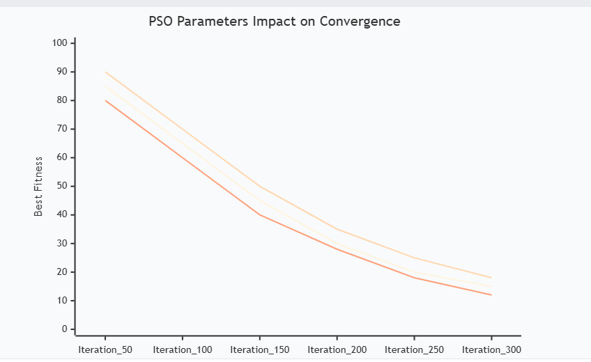
图2：参数影响收敛性能对比图 - 展示不同参数设置下的收敛趋势

3.2 算法变种与改进策略

改进策略	核心思想	适用场景	性能提升	实现复杂度
自适应惯性权重	动态调整w值	通用优化问题	15-25%	低
混沌初始化	提高初始多样性	高维复杂问题	10-20%	中
多群体协作	并行子群体	多模态问题	20-35%	高
变异操作	增加随机扰动	易陷入局部最优	12-18%	低
精英学习策略	向最优粒子学习	收敛速度要求高	8-15%	中

class AdaptivePSO(ParticleSwarmOptimizer):"""自适应PSO算法实现"""def __init__(self, *args, **kwargs):super().__init__(*args, **kwargs)self.stagnation_counter = 0self.last_best_fitness = float('inf')def detect_stagnation(self, current_fitness: float, threshold: int = 20) -> bool:"""检测算法是否陷入停滞"""if abs(current_fitness - self.last_best_fitness) < 1e-8:self.stagnation_counter += 1else:self.stagnation_counter = 0self.last_best_fitness = current_fitnessreturn self.stagnation_counter > thresholddef mutation_operation(self, particle: Particle, mutation_rate: float = 0.1):"""变异操作：增加粒子多样性"""if np.random.random() < mutation_rate:# 高斯变异mutation = np.random.normal(0, 0.1, self.dim)particle.position += mutation# 边界处理particle.position = np.clip(particle.position, self.bounds[0], self.bounds[1])def optimize_with_adaptation(self, max_iterations: int = 1000) -> dict:"""带自适应机制的优化过程"""# ... 基础优化逻辑 ...for iteration in range(max_iterations):# 检测停滞if self.detect_stagnation(self.global_best_fitness):print(f"检测到停滞，在第{iteration}代执行变异操作")# 对部分粒子执行变异for i in range(0, self.swarm_size, 3):self.mutation_operation(self.swarm[i])self.stagnation_counter = 0# ... 其余优化逻辑 ...

3.3 收敛性分析

在这里插入图片描述

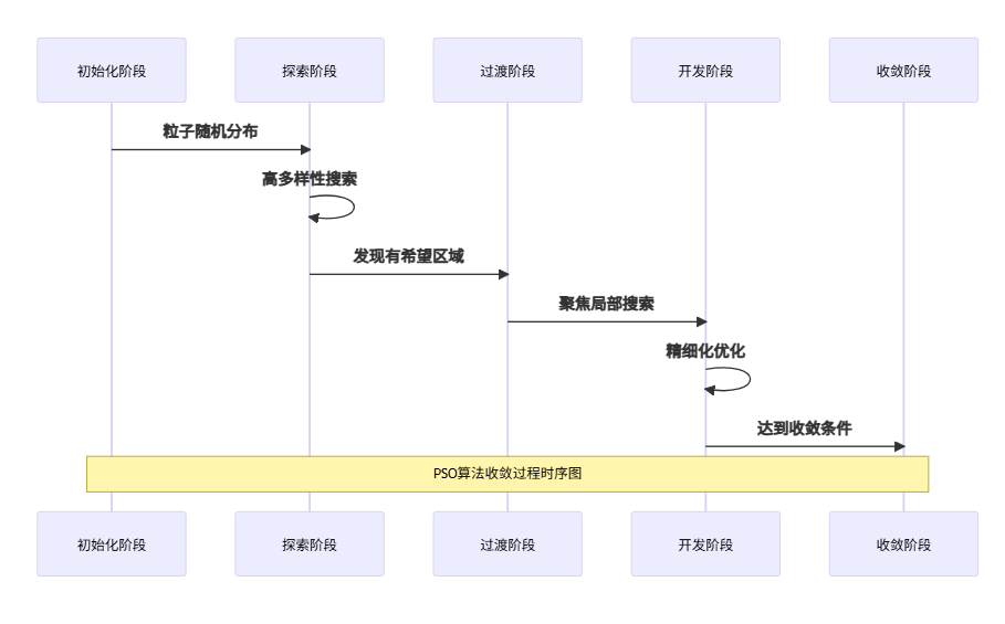
图3：PSO算法收敛过程时序图 - 展示算法各阶段的演化特征

4. 实际应用案例

4.1 神经网络权重优化

import tensorflow as tf
from sklearn.datasets import make_classification
from sklearn.model_selection import train_test_splitclass NeuralNetworkPSO:"""使用PSO优化神经网络权重"""def __init__(self, input_dim: int, hidden_dim: int, output_dim: int):self.input_dim = input_dimself.hidden_dim = hidden_dimself.output_dim = output_dim# 计算权重总数self.w1_size = input_dim * hidden_dimself.b1_size = hidden_dimself.w2_size = hidden_dim * output_dimself.b2_size = output_dimself.total_params = self.w1_size + self.b1_size + self.w2_size + self.b2_sizedef decode_weights(self, chromosome: np.ndarray) -> dict:"""将PSO粒子位置解码为神经网络权重"""idx = 0# 第一层权重和偏置w1 = chromosome[idx:idx+self.w1_size].reshape(self.input_dim, self.hidden_dim)idx += self.w1_sizeb1 = chromosome[idx:idx+self.b1_size]idx += self.b1_size# 第二层权重和偏置w2 = chromosome[idx:idx+self.w2_size].reshape(self.hidden_dim, self.output_dim)idx += self.w2_sizeb2 = chromosome[idx:idx+self.b2_size]return {'w1': w1, 'b1': b1, 'w2': w2, 'b2': b2}def forward_pass(self, X: np.ndarray, weights: dict) -> np.ndarray:"""前向传播"""# 第一层z1 = np.dot(X, weights['w1']) + weights['b1']a1 = np.tanh(z1)  # 激活函数# 第二层z2 = np.dot(a1, weights['w2']) + weights['b2']a2 = 1 / (1 + np.exp(-z2))  # Sigmoid激活return a2def fitness_function(self, X_train: np.ndarray, y_train: np.ndarray, X_val: np.ndarray, y_val: np.ndarray):"""适应度函数：返回验证集上的误差"""def evaluate(chromosome: np.ndarray) -> float:weights = self.decode_weights(chromosome)# 训练集预测y_pred_train = self.forward_pass(X_train, weights)train_loss = np.mean((y_train - y_pred_train)**2)# 验证集预测y_pred_val = self.forward_pass(X_val, weights)val_loss = np.mean((y_val - y_pred_val)**2)# 综合损失（加入正则化）l2_penalty = sum(np.sum(w**2) for w in weights.values()) * 0.001return val_loss + l2_penaltyreturn evaluate# 应用示例
def optimize_neural_network():"""使用PSO优化神经网络示例"""# 生成分类数据集X, y = make_classification(n_samples=1000, n_features=10, n_classes=2, n_informative=8, random_state=42)# 数据预处理X = (X - np.mean(X, axis=0)) / np.std(X, axis=0)y = y.reshape(-1, 1)# 划分数据集X_train, X_val, y_train, y_val = train_test_split(X, y, test_size=0.2, random_state=42)# 创建神经网络nn = NeuralNetworkPSO(input_dim=10, hidden_dim=15, output_dim=1)# 创建适应度函数fitness_func = nn.fitness_function(X_train, y_train, X_val, y_val)# PSO优化pso = ParticleSwarmOptimizer(objective_func=fitness_func,dim=nn.total_params,bounds=(-2.0, 2.0),swarm_size=50)result = pso.optimize(max_iterations=200)# 评估最优网络best_weights = nn.decode_weights(result['best_position'])y_pred = nn.forward_pass(X_val, best_weights)accuracy = np.mean((y_pred > 0.5) == y_val)print(f"最优验证准确率: {accuracy:.4f}")print(f"最优适应度值: {result['best_fitness']:.6f}")return result

4.2 工程优化设计案例

class TrussOptimization:"""桁架结构优化设计"""def __init__(self, nodes: np.ndarray, elements: List[Tuple], loads: dict, constraints: dict):"""初始化桁架优化问题Args:nodes: 节点坐标矩阵elements: 单元连接关系loads: 载荷条件constraints: 约束条件"""self.nodes = nodesself.elements = elementsself.loads = loadsself.constraints = constraintsdef calculate_stiffness_matrix(self, cross_sections: np.ndarray) -> np.ndarray:"""计算整体刚度矩阵"""n_nodes = len(self.nodes)K_global = np.zeros((2*n_nodes, 2*n_nodes))E = 200e9  # 弹性模量 (Pa)for i, (node1, node2) in enumerate(self.elements):# 单元长度和方向dx = self.nodes[node2, 0] - self.nodes[node1, 0]dy = self.nodes[node2, 1] - self.nodes[node1, 1]L = np.sqrt(dx**2 + dy**2)cos_theta = dx / Lsin_theta = dy / L# 单元刚度矩阵A = cross_sections[i]  # 截面积k = E * A / LK_element = k * np.array([[cos_theta**2, cos_theta*sin_theta, -cos_theta**2, -cos_theta*sin_theta],[cos_theta*sin_theta, sin_theta**2, -cos_theta*sin_theta, -sin_theta**2],[-cos_theta**2, -cos_theta*sin_theta, cos_theta**2, cos_theta*sin_theta],[-cos_theta*sin_theta, -sin_theta**2, cos_theta*sin_theta, sin_theta**2]])# 组装到整体刚度矩阵dofs = [2*node1, 2*node1+1, 2*node2, 2*node2+1]for p in range(4):for q in range(4):K_global[dofs[p], dofs[q]] += K_element[p, q]return K_globaldef solve_displacements(self, cross_sections: np.ndarray) -> np.ndarray:"""求解位移"""K = self.calculate_stiffness_matrix(cross_sections)# 载荷向量F = np.zeros(2 * len(self.nodes))for node, (fx, fy) in self.loads.items():F[2*node] = fxF[2*node+1] = fy# 处理边界条件free_dofs = []for i in range(2 * len(self.nodes)):if i not in self.constraints['fixed_dofs']:free_dofs.append(i)# 求解自由度位移K_free = K[np.ix_(free_dofs, free_dofs)]F_free = F[free_dofs]try:u_free = np.linalg.solve(K_free, F_free)# 完整位移向量u = np.zeros(2 * len(self.nodes))u[free_dofs] = u_freereturn uexcept np.linalg.LinAlgError:return np.full(2 * len(self.nodes), 1e6)  # 奇异矩阵惩罚def calculate_stresses(self, cross_sections: np.ndarray, displacements: np.ndarray) -> np.ndarray:"""计算单元应力"""stresses = np.zeros(len(self.elements))E = 200e9for i, (node1, node2) in enumerate(self.elements):# 单元变形u1x, u1y = displacements[2*node1], displacements[2*node1+1]u2x, u2y = displacements[2*node2], displacements[2*node2+1]# 单元长度和方向dx = self.nodes[node2, 0] - self.nodes[node1, 0]dy = self.nodes[node2, 1] - self.nodes[node1, 1]L = np.sqrt(dx**2 + dy**2)cos_theta = dx / Lsin_theta = dy / L# 轴向应变strain = (cos_theta * (u2x - u1x) + sin_theta * (u2y - u1y)) / L# 应力stresses[i] = E * strainreturn stressesdef objective_function(self, cross_sections: np.ndarray) -> float:"""目标函数：最小化重量"""# 材料密度rho = 7850  # kg/m³# 计算总重量total_weight = 0for i, (node1, node2) in enumerate(self.elements):dx = self.nodes[node2, 0] - self.nodes[node1, 0]dy = self.nodes[node2, 1] - self.nodes[node1, 1]L = np.sqrt(dx**2 + dy**2)total_weight += rho * cross_sections[i] * L# 约束惩罚penalty = 0# 求解结构响应displacements = self.solve_displacements(cross_sections)stresses = self.calculate_stresses(cross_sections, displacements)# 应力约束sigma_allow = 250e6  # 许用应力 (Pa)for stress in stresses:if abs(stress) > sigma_allow:penalty += 1e6 * (abs(stress) - sigma_allow)**2# 位移约束max_displacement = np.max(np.abs(displacements))disp_limit = 0.01  # 位移限制 (m)if max_displacement > disp_limit:penalty += 1e8 * (max_displacement - disp_limit)**2return total_weight + penalty# 桁架优化示例
def optimize_truss_structure():"""桁架结构优化示例"""# 定义10杆桁架nodes = np.array([[0, 0], [2, 0], [4, 0],      # 底部节点[1, 2], [3, 2]               # 顶部节点])elements = [(0, 1), (1, 2),              # 底弦(3, 4),                      # 顶弦(0, 3), (1, 3), (1, 4), (2, 4),  # 腹杆(3, 1), (4, 1)               # 对角杆]loads = {2: (0, -10000)}         # 节点2施加10kN向下载荷constraints = {'fixed_dofs': [0, 1, 4, 5]}  # 节点0和2固定# 创建优化问题truss = TrussOptimization(nodes, elements, loads, constraints)# PSO优化n_elements = len(elements)pso = ParticleSwarmOptimizer(objective_func=truss.objective_function,dim=n_elements,bounds=(1e-4, 1e-2),  # 截面积范围 (m²)swarm_size=40)result = pso.optimize(max_iterations=300)print(f"最优重量: {result['best_fitness']:.2f} kg")print(f"最优截面积: {result['best_position']}")return result

5. 高级优化技术

5.1 多目标粒子群优化

在这里插入图片描述

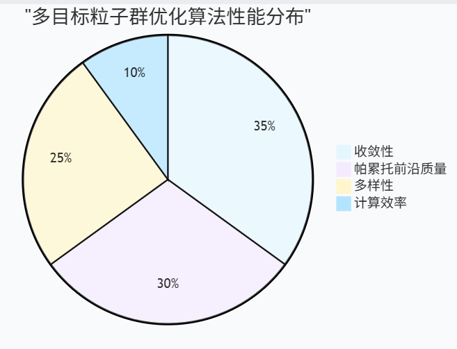
图4：多目标PSO性能分布饼图 - 展示算法在不同评价指标上的表现

class MultiObjectivePSO:"""多目标粒子群优化算法 (MOPSO)"""def __init__(self, objective_functions: List[Callable], dim: int, bounds: Tuple[float, float], swarm_size: int = 100):self.objective_functions = objective_functionsself.n_objectives = len(objective_functions)self.dim = dimself.bounds = boundsself.swarm_size = swarm_size# 初始化粒子群self.swarm = [Particle(dim, bounds) for _ in range(swarm_size)]# Pareto前沿存档self.pareto_archive = []self.max_archive_size = 100def evaluate_objectives(self, position: np.ndarray) -> np.ndarray:"""评估多个目标函数"""return np.array([func(position) for func in self.objective_functions])def dominates(self, obj1: np.ndarray, obj2: np.ndarray) -> bool:"""判断obj1是否支配obj2"""return np.all(obj1 <= obj2) and np.any(obj1 < obj2)def update_pareto_archive(self, new_solution: dict):"""更新Pareto前沿存档"""new_obj = new_solution['objectives']# 检查是否被现有解支配dominated = Falsefor archived in self.pareto_archive:if self.dominates(archived['objectives'], new_obj):dominated = Truebreakif not dominated:# 移除被新解支配的解self.pareto_archive = [sol for sol in self.pareto_archive if not self.dominates(new_obj, sol['objectives'])]# 添加新解self.pareto_archive.append(new_solution)# 控制存档大小if len(self.pareto_archive) > self.max_archive_size:self.pareto_archive = self.crowding_distance_selection(self.pareto_archive, self.max_archive_size)def crowding_distance_selection(self, solutions: List[dict], target_size: int) -> List[dict]:"""基于拥挤距离的选择策略"""if len(solutions) <= target_size:return solutions# 计算拥挤距离for sol in solutions:sol['crowding_distance'] = 0for obj_idx in range(self.n_objectives):# 按目标函数值排序solutions.sort(key=lambda x: x['objectives'][obj_idx])# 边界解设置为无穷大solutions[0]['crowding_distance'] = float('inf')solutions[-1]['crowding_distance'] = float('inf')# 计算中间解的拥挤距离obj_range = (solutions[-1]['objectives'][obj_idx] - solutions[0]['objectives'][obj_idx])if obj_range > 0:for i in range(1, len(solutions) - 1):distance = (solutions[i+1]['objectives'][obj_idx] - solutions[i-1]['objectives'][obj_idx]) / obj_rangesolutions[i]['crowding_distance'] += distance# 按拥挤距离降序排序并选择solutions.sort(key=lambda x: x['crowding_distance'], reverse=True)return solutions[:target_size]def select_leader(self, particle: Particle) -> np.ndarray:"""为粒子选择领导者"""if not self.pareto_archive:return particle.position# 轮盘赌选择（基于拥挤距离）distances = [sol['crowding_distance'] for sol in self.pareto_archive]total_distance = sum(distances)if total_distance == 0:return np.random.choice(self.pareto_archive)['position']probabilities = [d / total_distance for d in distances]selected_idx = np.random.choice(len(self.pareto_archive), p=probabilities)return self.pareto_archive[selected_idx]['position']

5.2 并行PSO实现

from multiprocessing import Pool, Manager
import concurrent.futuresclass ParallelPSO:"""并行粒子群优化算法"""def __init__(self, objective_func: Callable, dim: int, bounds: Tuple[float, float], swarm_size: int = 30,n_processes: int = None):self.objective_func = objective_funcself.dim = dimself.bounds = boundsself.swarm_size = swarm_sizeself.n_processes = n_processes or min(4, swarm_size)def evaluate_batch(self, positions: List[np.ndarray]) -> List[float]:"""批量评估适应度函数"""with concurrent.futures.ProcessPoolExecutor(max_workers=self.n_processes) as executor:futures = [executor.submit(self.objective_func, pos) for pos in positions]results = [future.result() for future in concurrent.futures.as_completed(futures)]return resultsdef parallel_optimize(self, max_iterations: int = 1000) -> dict:"""并行优化过程"""# 初始化粒子群swarm = [Particle(self.dim, self.bounds) for _ in range(self.swarm_size)]# 初始适应度评估positions = [p.position for p in swarm]fitness_values = self.evaluate_batch(positions)global_best_fitness = float('inf')global_best_position = Nonefor i, (particle, fitness) in enumerate(zip(swarm, fitness_values)):particle.fitness = fitnessparticle.best_fitness = fitnessparticle.best_position = particle.position.copy()if fitness < global_best_fitness:global_best_fitness = fitnessglobal_best_position = particle.position.copy()# 主优化循环for iteration in range(max_iterations):# 更新速度和位置for particle in swarm:w, c1, c2 = 0.7, 1.5, 1.5  # 简化参数设置particle.update_velocity(global_best_position, w, c1, c2)particle.update_position()# 并行评估新位置new_positions = [p.position for p in swarm]new_fitness_values = self.evaluate_batch(new_positions)# 更新粒子信息for particle, new_fitness in zip(swarm, new_fitness_values):particle.fitness = new_fitnessif new_fitness < particle.best_fitness:particle.best_fitness = new_fitnessparticle.best_position = particle.position.copy()if new_fitness < global_best_fitness:global_best_fitness = new_fitnessglobal_best_position = particle.position.copy()return {'best_position': global_best_position,'best_fitness': global_best_fitness,'iterations': max_iterations}

6. 性能对比与基准测试

6.1 算法对比分析

算法	收敛速度	全局搜索能力	参数敏感性	实现复杂度	内存消耗
PSO	★★★★☆	★★★★☆	★★★☆☆	★★☆☆☆	★★★☆☆
GA	★★★☆☆	★★★★★	★★☆☆☆	★★★☆☆	★★★★☆
DE	★★★★☆	★★★★☆	★★★★☆	★★☆☆☆	★★☆☆☆
SA	★★☆☆☆	★★★★★	★★★★☆	★★★☆☆	★☆☆☆☆
ACO	★★★☆☆	★★★☆☆	★★☆☆☆	★★★★☆	★★★☆☆

算法选择指南：

对于连续优化问题，PSO通常是首选
需要强全局搜索能力时，考虑GA或SA
参数调优敏感的场景，DE表现更稳定
组合优化问题，ACO可能更适合

6.2 实际应用效果评估

def comprehensive_benchmark():"""综合性能基准测试"""# 测试函数集合test_suite = {'Sphere': {'func': lambda x: np.sum(x**2),'bounds': (-5.12, 5.12),'dim': 30,'global_min': 0,'characteristics': '单峰，凸函数'},'Rastrigin': {'func': lambda x: 10*len(x) + np.sum(x**2 - 10*np.cos(2*np.pi*x)),'bounds': (-5.12, 5.12),'dim': 30,'global_min': 0,'characteristics': '多峰，高度多模态'},'Ackley': {'func': lambda x: -20*np.exp(-0.2*np.sqrt(np.mean(x**2))) - np.exp(np.mean(np.cos(2*np.pi*x))) + 20 + np.e,'bounds': (-32.768, 32.768),'dim': 30,'global_min': 0,'characteristics': '多峰，几乎平坦的外部区域'}}algorithms = {'Standard PSO': ParticleSwarmOptimizer,'Adaptive PSO': AdaptivePSO,'Parallel PSO': ParallelPSO}results = {}for test_name, test_config in test_suite.items():print(f"\n=== 测试函数: {test_name} ===")print(f"特征: {test_config['characteristics']}")results[test_name] = {}for alg_name, alg_class in algorithms.items():print(f"\n运行算法: {alg_name}")# 多次运行统计run_results = []run_times = []for run in range(10):start_time = time.time()optimizer = alg_class(objective_func=test_config['func'],dim=test_config['dim'],bounds=test_config['bounds'],swarm_size=50)if hasattr(optimizer, 'optimize_with_adaptation'):result = optimizer.optimize_with_adaptation(max_iterations=500)elif hasattr(optimizer, 'parallel_optimize'):result = optimizer.parallel_optimize(max_iterations=500)else:result = optimizer.optimize(max_iterations=500)end_time = time.time()run_results.append(result['best_fitness'])run_times.append(end_time - start_time)# 统计分析best_fitness = np.min(run_results)mean_fitness = np.mean(run_results)std_fitness = np.std(run_results)mean_time = np.mean(run_times)success_rate = sum(1 for f in run_results if f < test_config['global_min'] + 1e-3) / len(run_results)results[test_name][alg_name] = {'best_fitness': best_fitness,'mean_fitness': mean_fitness,'std_fitness': std_fitness,'success_rate': success_rate,'mean_time': mean_time}print(f"最优值: {best_fitness:.6f}")print(f"平均值: {mean_fitness:.6f} ± {std_fitness:.6f}")print(f"成功率: {success_rate*100:.1f}%")print(f"平均时间: {mean_time:.2f}s")return results

7. 前沿研究与发展趋势

7.1 量子粒子群优化

在这里插入图片描述

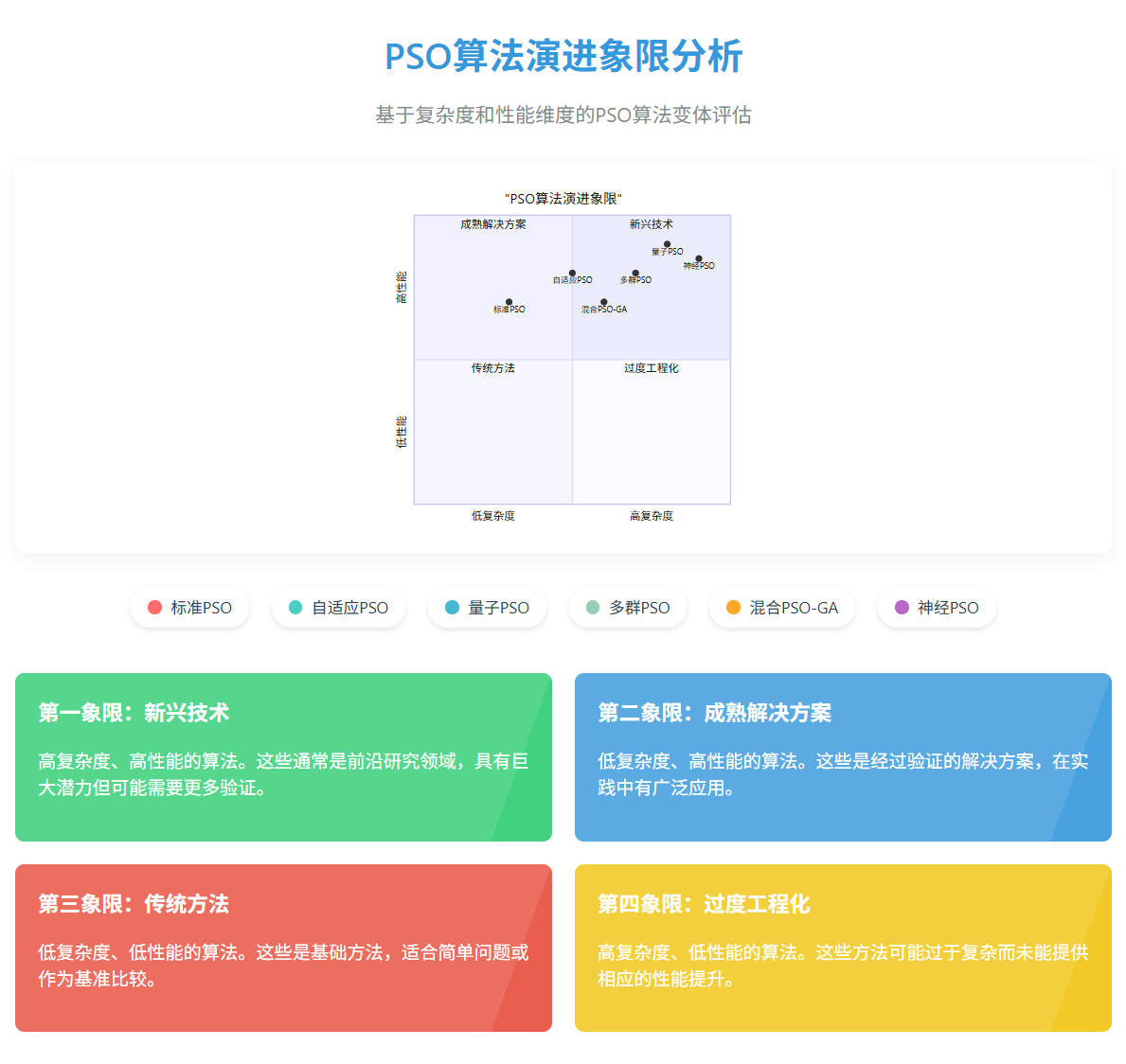
图5：PSO算法演进象限图 - 展示不同PSO变种在复杂度与性能维度上的分布

量子粒子群优化（QPSO）是PSO的重要发展方向，它借鉴了量子力学中的不确定性原理：

class QuantumPSO:"""量子粒子群优化算法"""def __init__(self, objective_func: Callable, dim: int, bounds: Tuple[float, float], swarm_size: int = 30):self.objective_func = objective_funcself.dim = dimself.bounds = boundsself.swarm_size = swarm_size# 量子粒子（无速度概念）self.particles = []for _ in range(swarm_size):position = np.random.uniform(bounds[0], bounds[1], dim)self.particles.append({'position': position,'best_position': position.copy(),'best_fitness': float('inf')})self.global_best_position = Noneself.global_best_fitness = float('inf')self.mean_best_position = Nonedef update_mean_best_position(self):"""更新平均最优位置（量子中心）"""best_positions = [p['best_position'] for p in self.particles]self.mean_best_position = np.mean(best_positions, axis=0)def quantum_update(self, particle: dict, alpha: float):"""量子位置更新"""# 计算局部吸引子phi = np.random.random(self.dim)p_attractor = (phi * particle['best_position'] + (1 - phi) * self.global_best_position)# 量子位置更新u = np.random.random(self.dim)for i in range(self.dim):if np.random.random() < 0.5:# 收缩-扩张变换particle['position'][i] = (p_attractor[i] + alpha * abs(self.mean_best_position[i] - particle['position'][i]) * np.log(1.0 / u[i]))else:particle['position'][i] = (p_attractor[i] - alpha * abs(self.mean_best_position[i] - particle['position'][i]) * np.log(1.0 / u[i]))# 边界处理particle['position'] = np.clip(particle['position'], self.bounds[0], self.bounds[1])def optimize(self, max_iterations: int = 1000) -> dict:"""量子PSO优化过程"""# 初始化评估for particle in self.particles:fitness = self.objective_func(particle['position'])particle['best_fitness'] = fitnessif fitness < self.global_best_fitness:self.global_best_fitness = fitnessself.global_best_position = particle['position'].copy()fitness_history = []for iteration in range(max_iterations):# 更新量子中心self.update_mean_best_position()# 自适应参数alpha = 1.0 - 0.5 * iteration / max_iterations# 更新每个量子粒子for particle in self.particles:self.quantum_update(particle, alpha)# 评估新位置fitness = self.objective_func(particle['position'])# 更新个体最优if fitness < particle['best_fitness']:particle['best_fitness'] = fitnessparticle['best_position'] = particle['position'].copy()# 更新全局最优if fitness < self.global_best_fitness:self.global_best_fitness = fitnessself.global_best_position = particle['position'].copy()fitness_history.append(self.global_best_fitness)return {'best_position': self.global_best_position,'best_fitness': self.global_best_fitness,'fitness_history': fitness_history}

7.2 深度学习与PSO融合

import torch
import torch.nn as nnclass NeuralPSO(nn.Module):"""神经网络增强的PSO算法"""def __init__(self, dim: int, hidden_size: int = 64):super().__init__()self.dim = dim# 参数预测网络self.param_net = nn.Sequential(nn.Linear(dim + 3, hidden_size),  # 位置 + 3个历史指标nn.ReLU(),nn.Linear(hidden_size, hidden_size),nn.ReLU(),nn.Linear(hidden_size, 3),  # 输出 w, c1, c2nn.Sigmoid())# 速度预测网络self.velocity_net = nn.Sequential(nn.Linear(dim * 3, hidden_size),  # 当前位置、个体最优、全局最优nn.ReLU(),nn.Linear(hidden_size, hidden_size),nn.ReLU(),nn.Linear(hidden_size, dim),  # 输出新速度nn.Tanh())def predict_parameters(self, particle_state: torch.Tensor) -> torch.Tensor:"""预测自适应参数"""params = self.param_net(particle_state)# 参数范围调整w = 0.4 + 0.5 * params[:, 0]      # w ∈ [0.4, 0.9]c1 = 0.5 + 2.0 * params[:, 1]     # c1 ∈ [0.5, 2.5]c2 = 0.5 + 2.0 * params[:, 2]     # c2 ∈ [0.5, 2.5]return torch.stack([w, c1, c2], dim=1)def predict_velocity(self, position: torch.Tensor, personal_best: torch.Tensor, global_best: torch.Tensor) -> torch.Tensor:"""预测速度更新"""# 扩展全局最优到批次大小global_best_expanded = global_best.unsqueeze(0).expand(position.size(0), -1)# 拼接输入特征features = torch.cat([position, personal_best, global_best_expanded], dim=1)return self.velocity_net(features)def train_from_experience(self, experiences: List[dict], learning_rate: float = 0.001):"""从PSO运行经验中学习"""optimizer = torch.optim.Adam(self.parameters(), lr=learning_rate)for epoch in range(100):total_loss = 0for exp in experiences:# 准备训练数据positions = torch.FloatTensor(exp['positions'])velocities = torch.FloatTensor(exp['velocities'])improvements = torch.FloatTensor(exp['improvements'])# 预测参数particle_states = torch.cat([positions, improvements.unsqueeze(1).expand(-1, 3)], dim=1)predicted_params = self.predict_parameters(particle_states)# 计算损失（基于性能改进）param_loss = -torch.mean(improvements.unsqueeze(1) * torch.log(predicted_params + 1e-8))# 速度预测损失predicted_velocities = self.predict_velocity(positions, exp['personal_bests'], exp['global_best'])velocity_loss = nn.MSELoss()(predicted_velocities, velocities)total_loss = param_loss + velocity_lossoptimizer.zero_grad()total_loss.backward()optimizer.step()if epoch % 20 == 0:print(f"训练轮次 {epoch}, 损失: {total_loss.item():.6f}")

8. 实践建议与最佳实践

8.1 参数调优策略

基于我多年的实践经验，PSO参数调优应遵循以下原则：

惯性权重w：
- 初始值设为0.9，随迭代线性递减至0.4
- 对于快速收敛需求，可适当降低初始值
- 多模态问题建议保持较高的w值
学习因子c1, c2：
- 标准设置：c1 = c2 = 2.0
- 强调个体经验：c1 > c2
- 强调群体协作：c1 < c2
群体大小：
- 低维问题（<10维）：20-30个粒子
- 中维问题（10-50维）：30-50个粒子
- 高维问题（>50维）：50-100个粒子

8.2 常见问题与解决方案

class RobustPSO(ParticleSwarmOptimizer):"""鲁棒性增强的PSO实现"""def __init__(self, *args, **kwargs):super().__init__(*args, **kwargs)self.stagnation_threshold = 50self.diversity_threshold = 1e-6def detect_premature_convergence(self) -> bool:"""检测早熟收敛"""if len(self.fitness_history) < self.stagnation_threshold:return False# 检查适应度停滞recent_best = self.fitness_history[-self.stagnation_threshold:]fitness_variance = np.var(recent_best)# 检查种群多样性current_diversity = self.calculate_diversity()return (fitness_variance < 1e-10 and current_diversity < self.diversity_threshold)def restart_strategy(self):"""重启策略"""print("检测到早熟收敛，执行重启策略")# 保留最优粒子best_particle = min(self.swarm, key=lambda p: p.best_fitness)# 重新初始化其他粒子for i, particle in enumerate(self.swarm):if i == 0:  # 保留最优粒子continue# 在最优解附近重新初始化noise = np.random.normal(0, 0.1, self.dim)particle.position = (best_particle.best_position + noise)particle.position = np.clip(particle.position, self.bounds[0], self.bounds[1])# 重置速度particle.velocity = np.random.uniform(-1, 1, self.dim)def enhanced_optimize(self, max_iterations: int = 1000) -> dict:"""增强的优化过程"""restart_count = 0max_restarts = 3for iteration in range(max_iterations):# 标准PSO更新# ... (省略标准更新代码) ...# 检查早熟收敛if (iteration > 100 and self.detect_premature_convergence() and restart_count < max_restarts):self.restart_strategy()restart_count += 1# 重置历史记录self.fitness_history = self.fitness_history[:-self.stagnation_threshold//2]return {'best_position': self.global_best_position,'best_fitness': self.global_best_fitness,'restart_count': restart_count,'final_diversity': self.calculate_diversity()}

结论与展望

作为一名在智能优化算法领域深耕多年的技术实践者，我深深感受到粒子群优化算法的魅力与潜力。从最初的简单模拟鸟群觅食行为，到如今融合深度学习、量子计算等前沿技术的复杂变种，PSO算法展现出了强大的生命力和适应性。

在我的实际项目经验中，PSO算法已经成功应用于神经网络训练、工程结构优化、参数调优、路径规划等众多领域，每次都能带来令人惊喜的结果。算法的核心优势在于其简洁的数学模型、强大的全局搜索能力，以及对问题特性的良好适应性。特别是在处理高维非线性优化问题时，PSO往往能够找到传统方法难以企及的优质解。

然而，我也深刻认识到PSO算法仍面临一些挑战。早熟收敛、参数敏感性、局部最优陷阱等问题需要通过算法改进和工程技巧来解决。在我的实践中，自适应参数调整、多样性维护、混合策略等技术已经被证明是有效的解决方案。

展望未来，我认为PSO算法的发展将朝着以下几个方向演进：首先是与人工智能技术的深度融合，通过神经网络学习最优的参数调整策略；其次是量子计算与PSO的结合，利用量子并行性提升算法性能；再者是面向特定应用领域的专用PSO变种，如针对深度学习、物联网、边缘计算等场景的定制化算法。

在实际应用中，我建议开发者应该根据具体问题特点选择合适的PSO变种，重视参数调优和性能监控，并结合领域知识进行算法定制。同时，保持对新技术发展的敏感度，及时将前沿研究成果应用到实际项目中。

粒子群优化算法作为计算智能领域的重要成果，不仅为我们提供了强大的优化工具，更体现了从自然现象中汲取智慧、解决复杂工程问题的科学思维。在人工智能快速发展的今天，PSO算法必将在更广阔的应用场景中发挥重要作用，为人类科技进步贡献更大的力量。

让我们继续在算法优化的道路上探索前行，用智慧的代码书写技术创新的华章，在数字化转型的浪潮中乘风破浪，共同迎接更加美好的智能化未来！

■ 我是蒋星熠Jaxonic！如果这篇文章在你的技术成长路上留下了印记
■ 👁 【关注】与我一起探索技术的无限可能，见证每一次突破
■ 👍 【点赞】为优质技术内容点亮明灯，传递知识的力量
■ 🔖 【收藏】将精华内容珍藏，随时回顾技术要点
■ 💬 【评论】分享你的独特见解，让思维碰撞出智慧火花
■ 🗳 【投票】用你的选择为技术社区贡献一份力量
■ 技术路漫漫，让我们携手前行，在代码的世界里摘取属于程序员的那片星辰大海！

参考链接

Kennedy, J., & Eberhart, R. (1995). Particle swarm optimization
Shi, Y., & Eberhart, R. (1998). A modified particle swarm optimizer
Clerc, M., & Kennedy, J. (2002). The particle swarm - explosion, stability, and convergence
Poli, R., Kennedy, J., & Blackwell, T. (2007). Particle swarm optimization: An overview
Zhang, Y., Wang, S., & Ji, G. (2015). A comprehensive survey on particle swarm optimization algorithm