EPWpy教程:一个脚本完成能带、声子、电声耦合、弛豫时间计算

EPWpy 是一个开源 python 代码,它包装了 EPW 代码以进行自动计算,可使用 Quantum Espresso 和 EPW 自动执行 DFT+EPW 计算。同时还提供了一系列可视化实用程序,用于绘制各种数据和结果输出。
EPWpy安装可参考已有教程
EPWpy 安装教程
官网:https://epwpy.org
本文参考:https://epwpy.org/doc/notebooks/transport-v1.2.html
在本文中,使用从头开始玻尔兹曼输运方程(BTE)计算硅的声子有限载流子迁移率。基于jupyter notebook进行代码的分部步进运行,如需一次运行,请将全部代码和操作指令整合为单一脚本后运行。
定义环境。需配置MaterialsProjec API
import numpy as npimport matplotlib.pyplot as pltfrom matplotlib import rcimport time, sys, osimport pymatgen#from pymatgen.ext.matproj import MPResterfrom mp_api.client import MPRestermpr = MPRester(" ")import EPWpyfrom EPWpy import EPWpyfrom EPWpy.plotting import plot_bandsimport plotly.ioQE='/home/software/qe-7.1/bin'
定义基本函数
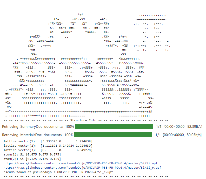
plotly.io.renderers.default = "sphinx_gallery"silicon=EPWpy.EPWpy({'prefix':'si','calculation':'\'scf\'','structure_mp':"mp-149",'ecutwfc':'40','celldm(1)':'10.262','pseudo_auto':True,},code=QE,env='mpirun')silicon.run_serial=True# Summarypseudopot=silicon.__dict__['pw_atomic_species']['pseudo'][0]print('Pseudopotential:', silicon.__dict__['pw_atomic_species']['pseudo'][0])print('Pseudopotential directory:', silicon.__dict__['pw_control']['pseudo_dir'])print('Prefix:',silicon.__dict__['prefix'])#app = silicon.display_lattice(supercell=[3,3,2],bond_length = 3.5,view={'in_notebook':True,'backend':'png'})#app
自洽(SCF) 计算
自洽计算,得到硅在基态下的电子电荷密度。计算包括三个独立的步骤:
1、指定siicon上SCF 计算的运行时参数。
2、根据步骤 1 中定义的属性以及 EPWpy 中默认设置的其他属性,创建 QE 所需的输入文件。
3、执行 SCF 计算
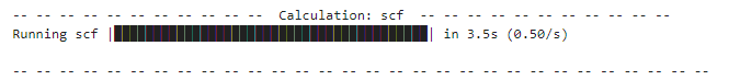
silicon.scf(name='scf',kpoints={'kpoints':[[6,6,6]]})silicon.prepare(1,type_run='scf')silicon.run(4)silicon.pw_util = silicon.PW_utilities()
能带结构计算
在这一步中沿着布里渊区的一些高对称线计算硅的能带结构。
silicon.scf(control={'calculation':'\'bands\''},system={'nbnd':12},kpoints={'kpoints':[['0.5','0.50','0.50','20'],['0.0','0.00','0.00','20'],['0.5','0.25','0.75','20']],'kpoints_type':'{crystal_b}'},name='bs')silicon.prepare(type_run='bs')silicon.run(4,type_run='bs')
能带结构图
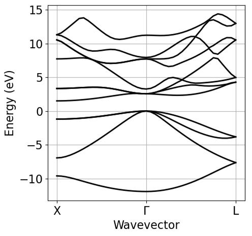
现在绘制了在上一步中计算的电子能带结构。能量轴的零点设置为通过 手动指定的值ef0
ef_from_file = silicon.pw_util.efermiBand=plot_bands.plot_band_scf(f'./{silicon.prefix}/bs/bs.out')plot_bands.plot_band_prod(Band,ef0=ef_from_file,xticks=['X','$\Gamma$','L'],xlabel = 'Wavevector',ylabel = 'Energy (eV)')
声子谱
计算声子有限的移动率,我们需要确定振动频率和特征模态。
第 1 步:均匀布里渊区网格上的声子计算
silicon.ph(phonons={'fildyn':'\'si.dyn\'','nq1':3,'nq2':3,'nq3':3,'fildvscf':'\'dvscf\''})silicon.prepare(type_run='ph')silicon.run(6,type_run='ph')
第 2 步:生成 IFC
silicon.q2r(name='q2r')silicon.prepare(type_run='q2r')silicon.run(1,type_run='q2r')
第 3 步:声子谱
调用执行matdyn.x
silicon.matdyn(name='matdyn',kpoints={'kpoints':[['0.5','0.50','0.50','20'],['0.0','0.00','0.00','20'],['0.5','0.25','0.75','20']],'kpoints_type':'{crystal_b}'},)silicon.prepare(type_run='matdyn')silicon.run(1,type_run='matdyn')
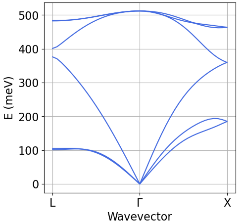
绘图
Band=plot_bands.plot_band_eig(f'./{silicon.prefix}/ph/si.freq')plot_bands.plot_band_freq(Band,ylabel='E (meV)',ef0=0,xticks=['L','$\Gamma$','X'],color='royalblue')
用EPW将电子和声子转化为Wannier基
在均匀布里渊区网格上计算Kohn-Sham方程
silicon.nscf(system={'nbnd':8},kpoints={'grid':[6,6,6],'kpoints_type': 'crystal'})silicon.prepare(type_run='nscf')silicon.run(4,type_run='nscf')
Bloch 转化为Wannier表象并保存
# File with k-path for sanity checkssilicon.epw(epwin={'wdata':['guiding_centres = .true.','dis_num_iter = 500','num_print_cycles = 10','dis_mix_ratio = 1','use_ws_distance = T'],'proj':['\'Si : sp3\''],'band_plot':'.true.','filkf':silicon.filkf_file,'filqf':silicon.filkf_file,'etf_mem':0,'fsthick':12.0,'wannierize':'.true.','elph':'.true.','num_iter':500},name='epw1')silicon.filkf_file = 'LGX.txt'silicon.filkf(path=[[0.5,0.5,0.5],[0.0,0.0,0.0],[0.5,0.25,0.75]],length=[51,51],)silicon.prepare(type_run='epw1')silicon.run(8,type_run='epw1')
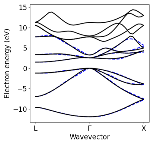
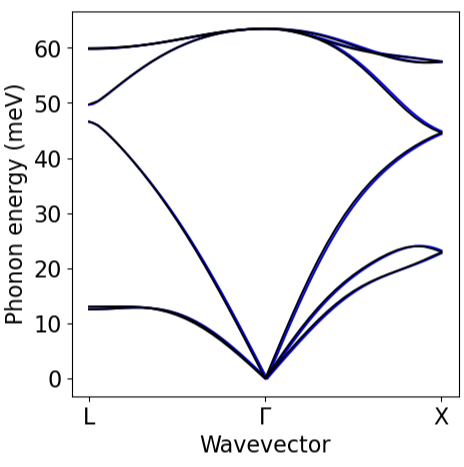
EPW 插值能带和声子,并绘图检查
# ElectronsBand_EPW=plot_bands.plot_band_eig(f'./{silicon.prefix}/epw/band.eig')Band_QE=plot_bands.plot_band_scf(f'./{silicon.prefix}/bs/bs.out')plot_bands.plot_band_prod(Band_EPW,ef0=ef_from_file,xlabel='Wavevector',ylabel='Electron energy (eV)',xticks=['L','$\Gamma$','X'],linestyle='--',color_c='b',color_v='b',first = True)plot_bands.plot_band_prod(Band_QE,ef0=ef_from_file,xlabel='Wavevector',ylabel='Electron energy (eV)',xticks=['L','$\Gamma$','X'],first = False) # False controls ifthis is the first set of plots# PhononsPH_epw=plot_bands.plot_band_eig(f'./{silicon.prefix}/epw/phband.freq')PH_matdyn=plot_bands.plot_band_eig(f'./{silicon.prefix}/ph/si.freq')PH_matdyn=PH_matdyn*0.124plot_bands.plot_band_freq(PH_epw,xlabel='Wavevector',ylabel='Phonon energy (meV)',ef0=0,xticks=['L','$\Gamma$','X'],linestyle='--',first = True,color='blue')plot_bands.plot_band_freq(PH_matdyn,xlabel='Wavevector',ylabel='Phonon energy (meV)',ef0=0,xticks=['L','$\Gamma$','X'],first = False)
载流子迁移率计算
#silicon.reset()silicon.epw(epwin={'elph':'.true.','etf_mem': '3','nkf1':40,'nkf2':40,'nkf3':40,'nqf1':40,'nqf2':40,'nqf3':40,'mp_mesh_k':'.true.','efermi_read':'.true.','fsthick': 0.3,'fermi_energy':6.5,'temps':'300 250 200 150 100','degaussw':0.0,'scattering':'.true.','int_mob':'.false.','carrier':'.true.','ncarrier' :'1E13','iterative_bte':'.true.','nstemp': 5,'clean_transport':None},name='epw2')silicon.prepare(type_run='epw2')silicon.run(6,type_run='epw2')

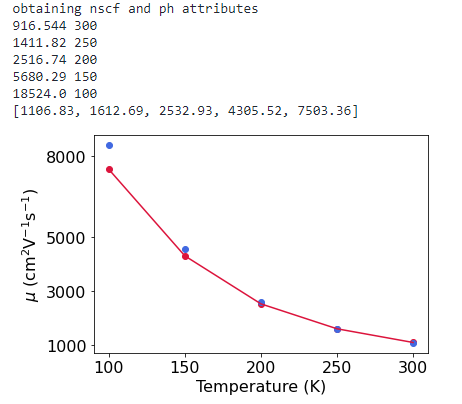
绘制迁移率结果
print(os.getcwd())silicon.reset()silicon.epw_fold = 'epw'silicon.epw_file = 'epw2'temps=[300, 250, 200, 150, 100]mob=[]font=16for T in temps:silicon.epw_params['temps']=Tprint(silicon.ibte_mobility_e[0,0],T)mob.append(silicon.ibte_mobility_e[1,1])plt.scatter(T,silicon.ibte_mobility_e[1,1], color = 'crimson')plt.scatter(T,silicon.serta_mobility_e[1,1], color = 'royalblue')print(mob)plt.plot(temps[::-1],mob[::-1], color = 'crimson')plt.xticks([100,150,200,250,300],fontsize=font)plt.yticks([1000,3000,5000,8000],fontsize=font)plt.xlabel('Temperature (K)',fontsize=16)plt.ylabel('$\mu$ (cm$^2$V$^{-1}$s$^{-1}$)',fontsize=16)plt.xticks(fontsize=16)plt.yticks(fontsize=16)plt.show()
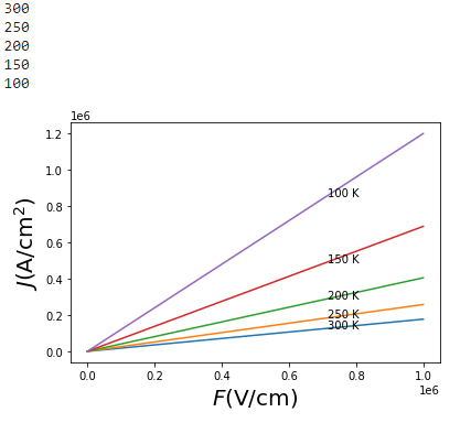
计算位移电流
![]()
E=np.linspace(0,1,50)*1e6 # V/cmn=1e15# cm^-3e = 1.6*10**-19 # CoulombJ = []for mu in mob:J.append(e*n*mu*E) # Ampere/cm^2for i,T in enumerate(temps):print(T)plt.plot(E,J[i])plt.text(E[-15],J[i][-15],str(T)+' K')plt.xlabel('$F \\rm (V/cm)$',fontsize=20)plt.ylabel('$J \\rm (A/cm^2)$',fontsize=20)plt.show()
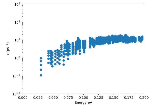
绘制弛豫时间
silicon.temp=400tau_inv=silicon.inv_taucbplt.scatter(tau_inv[:,3]-6.6,tau_inv[:,4])plt.yscale('log')plt.xlabel('Energy eV')plt.ylabel('$\\tau$ (ps$^{-1}$)')plt.axis([0,0.2,1e-2,1e3])plt.show()