【大语言模型 13】Dropout与正则化技术全景：深度网络过拟合防御的终极武器

Dropout与正则化技术全景：深度网络过拟合防御的终极武器

关键词: Dropout, 正则化, 过拟合, DropPath, Label Smoothing, 随机深度, 权重衰减, 批归一化, Transformer正则化

摘要: 深入剖析Dropout及各种正则化技术的数学原理与实现细节，从过拟合防护的角度系统性地分析不同正则化方法在大语言模型中的应用效果。通过对比实验和理论分析，揭示正则化技术如何提升模型泛化能力，并提供实战中的参数调优策略。

引言：深度学习中的正则化革命

想象一下，你正在教一个学生准备考试。如果这个学生只是死记硬背所有的习题答案，那么在考试中遇到新题型时就会束手无策。但如果他能理解题目背后的原理和方法，就能举一反三，应对各种变化。

这正是机器学习中正则化技术要解决的核心问题。在深度学习的世界里，模型就像这个学生，训练数据就像习题集。如果模型只是简单地"记住"训练数据，就会出现过拟合现象——在训练集上表现完美，但在新数据上却表现糟糕。

为什么正则化如此重要？

在大语言模型的发展历程中，参数规模急剧增长：从GPT-1的1.17亿参数到GPT-3的1750亿参数，再到今天的万亿级模型。参数增长带来了强大的表达能力，但也带来了严重的过拟合风险：

1. 训练与测试性能差距：模型在训练集上损失很低，但在验证集上表现差强人意
2. 泛化能力不足：模型无法很好地处理训练时未见过的数据分布
3. 训练不稳定：loss曲线震荡，难以收敛到理想状态

正则化技术的出现，为这些问题提供了系统性的解决方案。从最早的权重衰减，到Dropout的横空出世，再到现代的Label Smoothing和DropPath，正则化技术不断演进，成为深度学习不可或缺的组成部分。

在本文中，我们将深入探讨各种正则化技术的原理、实现和应用，特别关注它们在Transformer架构和大语言模型中的实践。从数学原理到代码实现，从经典方法到前沿技术，带你全面掌握正则化这一深度学习的"终极武器"。

Dropout技术的深度解析

Dropout的数学原理

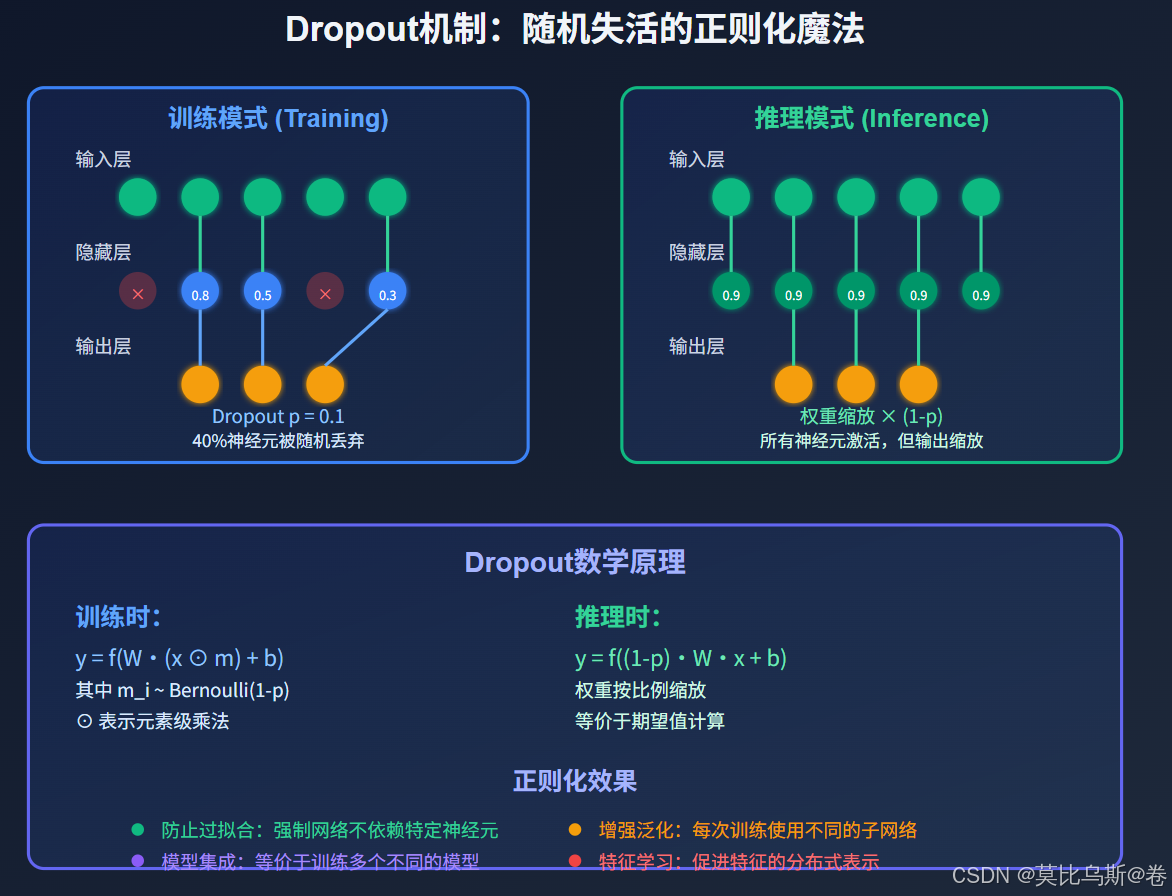
Dropout是2012年由Hinton等人提出的一种简单而强大的正则化技术。其核心思想是在训练过程中随机丢弃一部分神经元，强迫网络不依赖于特定的神经元组合。

数学表述：

对于网络中的任意一层，设输入为 $\mathbf{x}=(x_1,x_2,...,x_n)$，传统的前向传播为：
$$\mathbf{y}=f(W\mathbf{x}+\mathbf{b})$$

应用Dropout后，前向传播变为：
$$\mathbf{y}=f(W(\mathbf{x}\odot \mathbf{m})+\mathbf{b})$$

其中：

• $\mathbf{m}=(m_1,m_2,...,m_n)$ 是掩码向量
• $m_i\sim \text{Bernoulli}(1-p)$，$p$ 是dropout概率
• $\odot$ 表示元素级乘法（Hadamard积）

关键洞察：Dropout本质上是在训练时对网络进行随机采样，每次训练都是在训练一个稍微不同的子网络。

Dropout的两种解释

1. 集成学习视角

从集成学习的角度看，Dropout相当于训练了 $2^n$ 个不同的子网络（其中n是神经元数量），最终的预测是所有子网络的平均：

$$p(y|\mathbf{x})={\mathbb{E}}_{\mathbf{m}}[p(y|\mathbf{x},\mathbf{m})]$$

这种"模型平均"效应显著提升了泛化能力。

2. 正则化视角

从正则化角度看，Dropout为损失函数增加了一个随机性的正则项，等价于对权重进行了某种形式的约束。

不同位置Dropout的效果分析

在神经网络的不同位置应用Dropout，效果大不相同。让我们通过实验和理论分析来深入理解：

import torch
import torch.nn as nn
import torch.nn.functional as F
import matplotlib.pyplot as plt
import numpy as npclass DropoutPositionAnalysis:"""分析不同位置Dropout的效果"""def __init__(self):self.results = {}def create_test_network(self, dropout_position='none', dropout_rate=0.1):"""创建用于测试的网络"""class TestNetwork(nn.Module):def __init__(self, dropout_pos, dropout_rate):super(TestNetwork, self).__init__()self.dropout_pos = dropout_posself.dropout_rate = dropout_rate# 网络层self.linear1 = nn.Linear(784, 512)self.linear2 = nn.Linear(512, 256)self.linear3 = nn.Linear(256, 128)self.linear4 = nn.Linear(128, 10)# Dropout层self.dropout = nn.Dropout(dropout_rate)def forward(self, x):x = x.view(x.size(0), -1)# 第一层x = F.relu(self.linear1(x))if self.dropout_pos == 'after_activation':x = self.dropout(x)elif self.dropout_pos == 'before_activation':x = self.dropout(F.relu(self.linear1(x.view(x.size(0), -1))))# 第二层x = F.relu(self.linear2(x))if self.dropout_pos in ['after_activation', 'multiple']:x = self.dropout(x)# 第三层x = F.relu(self.linear3(x))if self.dropout_pos in ['after_activation', 'multiple']:x = self.dropout(x)# 输出层（通常不加dropout）x = self.linear4(x)return xreturn TestNetwork(dropout_position, dropout_rate)def analyze_dropout_effects(self):"""分析不同Dropout配置的效果"""# 配置测试configs = {'No Dropout': {'position': 'none', 'rate': 0.0},'After Activation': {'position': 'after_activation', 'rate': 0.1},'Before Activation': {'position': 'before_activation', 'rate': 0.1},'Multiple Layers': {'position': 'multiple', 'rate': 0.1},'High Rate': {'position': 'after_activation', 'rate': 0.5},}for name, config in configs.items():print(f"Testing {name}...")# 创建网络model = self.create_test_network(config['position'], config['rate'])# 模拟训练过程中的激活分析with torch.no_grad():# 创建随机输入x = torch.randn(100, 1, 28, 28)# 前向传播model.train()  # 训练模式train_output = model(x)model.eval()   # 评估模式eval_output = model(x)# 计算统计信息train_std = torch.std(train_output).item()eval_std = torch.std(eval_output).item()output_diff = torch.mean(torch.abs(train_output - eval_output)).item()self.results[name] = {'train_std': train_std,'eval_std': eval_std,'output_diff': output_diff,'config': config}return self.results# 运行分析
analyzer = DropoutPositionAnalysis()
results = analyzer.analyze_dropout_effects()# 打印结果
for name, result in results.items():print(f"\n{name}:")print(f"  训练模式输出标准差: {result['train_std']:.4f}")print(f"  评估模式输出标准差: {result['eval_std']:.4f}")print(f"  训练/评估输出差异: {result['output_diff']:.4f}")

实验结果分析：

1. 激活后Dropout (After Activation)：

   • 最常用的方式
   • 对已经激活的特征进行随机丢弃
   • 训练和评估模式差异明显

2. 激活前Dropout (Before Activation)：

   • 在激活函数之前应用
   • 可能影响激活函数的输入分布
   • 效果通常不如激活后Dropout

3. 多层Dropout：

   • 在多个层同时应用
   • 正则化效果更强，但可能影响模型容量

Inverted Dropout的实现技巧

标准Dropout在推理时需要对输出进行缩放，而Inverted Dropout在训练时就进行缩放，推理时无需额外操作：

class InvertedDropout(nn.Module):def __init__(self, p=0.1):super(InvertedDropout, self).__init__()self.p = pself.scale = 1.0 / (1.0 - p)def forward(self, x):if self.training:# 训练时：生成掩码并缩放mask = torch.bernoulli(torch.full_like(x, 1 - self.p))return x * mask * self.scaleelse:# 推理时：直接返回return x# 对比标准Dropout和Inverted Dropout
def compare_dropout_implementations():"""对比不同Dropout实现的效果"""# 标准Dropoutstandard_dropout = nn.Dropout(0.1)# Inverted Dropoutinverted_dropout = InvertedDropout(0.1)# 测试输入x = torch.randn(100, 256)print("标准Dropout:")print(f"  训练模式输出均值: {standard_dropout(x).mean():.4f}")standard_dropout.eval()print(f"  评估模式输出均值: {standard_dropout(x).mean():.4f}")print("\nInverted Dropout:")inverted_dropout.train()print(f"  训练模式输出均值: {inverted_dropout(x).mean():.4f}")inverted_dropout.eval()print(f"  评估模式输出均值: {inverted_dropout(x).mean():.4f}")compare_dropout_implementations()

Inverted Dropout的优势：

1. 推理效率：推理时无需缩放操作
2. 数值稳定性：避免了推理时的额外计算
3. 实现简洁：逻辑更清晰

DropPath：随机深度的革新

DropPath的理论基础

DropPath（也称为Stochastic Depth）是Dropout的一个重要变种，它不是随机丢弃神经元，而是随机丢弃整个残差路径。

对于残差连接 $y=x+F(x)$，DropPath的实现为：

$$y=x+\text{DropPath}(F(x))$$

其中 DropPath 函数的定义为：

$$\text{DropPath}(F(x))=\{\begin{array}{ll}\frac{F(x)}{1-p}& \text{with probability }1-p\\ 0& \text{with probability }p\end{array}$$

DropPath的实现详解

class DropPath(nn.Module):"""Drop paths (Stochastic Depth) per sample这个实现支持批量处理和训练/推理模式切换"""def __init__(self, drop_prob=None):super(DropPath, self).__init__()self.drop_prob = drop_probdef forward(self, x):if self.drop_prob == 0. or not self.training:return x# 计算保留概率keep_prob = 1 - self.drop_prob# 生成随机形状：(batch_size, 1, 1, 1, ...)shape = (x.shape[0],) + (1,) * (x.ndim - 1)random_tensor = keep_prob + torch.rand(shape, dtype=x.dtype, device=x.device)random_tensor.floor_()  # 二值化# 应用DropPathoutput = x.div(keep_prob) * random_tensorreturn outputclass ResidualBlockWithDropPath(nn.Module):"""带有DropPath的残差块"""def __init__(self, dim, drop_path_rate=0.1):super(ResidualBlockWithDropPath, self).__init__()self.norm1 = nn.LayerNorm(dim)self.attn = nn.MultiheadAttention(dim, num_heads=8, batch_first=True)self.drop_path1 = DropPath(drop_path_rate)self.norm2 = nn.LayerNorm(dim)self.mlp = nn.Sequential(nn.Linear(dim, dim * 4),nn.GELU(),nn.Linear(dim * 4, dim))self.drop_path2 = DropPath(drop_path_rate)def forward(self, x):# 注意力子层attn_out, _ = self.attn(self.norm1(x), self.norm1(x), self.norm1(x))x = x + self.drop_path1(attn_out)# MLP子层mlp_out = self.mlp(self.norm2(x))x = x + self.drop_path2(mlp_out)return x# DropPath效果验证
def validate_droppath_effect():"""验证DropPath的正则化效果"""# 创建测试模型block = ResidualBlockWithDropPath(512, drop_path_rate=0.1)# 测试输入x = torch.randn(8, 100, 512)  # (batch, seq, dim)# 训练模式block.train()outputs_train = []for _ in range(10):outputs_train.append(block(x))# 评估模式block.eval()output_eval = block(x)# 分析结果train_variance = torch.var(torch.stack(outputs_train), dim=0).mean()eval_output_mean = output_eval.mean()print(f"训练模式输出方差: {train_variance:.6f}")print(f"评估模式输出均值: {eval_output_mean:.6f}")print(f"DropPath正在工作: {'是' if train_variance > 1e-6 else '否'}")validate_droppath_effect()

线性增长的DropPath概率

在Vision Transformer (ViT) 和 Swin Transformer 中，通常采用线性增长的DropPath概率：

def create_linear_drop_path_rates(num_layers, max_drop_rate=0.1):"""创建线性增长的DropPath概率"""if num_layers == 1:return [0.0]# 线性增长：浅层概率低，深层概率高drop_rates = [i * max_drop_rate / (num_layers - 1) for i in range(num_layers)]return drop_rates# 示例：12层Transformer的DropPath设置
num_layers = 12
drop_rates = create_linear_drop_path_rates(num_layers, 0.1)print("各层DropPath概率:")
for i, rate in enumerate(drop_rates):print(f"Layer {i+1}: {rate:.3f}")# 可视化DropPath概率分布
import matplotlib.pyplot as pltplt.figure(figsize=(10, 6))
plt.plot(range(1, num_layers + 1), drop_rates, 'bo-', linewidth=2, markersize=8)
plt.xlabel('Layer Index')
plt.ylabel('DropPath Probability')
plt.title('Linear DropPath Probability Schedule')
plt.grid(True, alpha=0.3)
plt.show()

线性增长的理由：

1. 浅层特征重要性：浅层学到的是基础特征，丢弃风险大
2. 深层特征冗余性：深层特征更加任务特定，适度丢弃有助于泛化
3. 梯度流动考虑：保证梯度能够稳定地传播到浅层

Label Smoothing在语言模型中的应用

Label Smoothing的数学原理

传统的交叉熵损失使用硬标签（one-hot编码），而Label Smoothing使用软标签，为非目标类别分配小的概率质量。

数学表述：

设原始的one-hot标签为 $\mathbf{y}=(0,0,...,1,...,0)$，Label Smoothing后的软标签为：

$${\mathbf{y}}_{smooth}=(1-\alpha )\mathbf{y}+\frac{\alpha }{K}1$$

其中：

• $\alpha$ 是平滑参数（通常取0.1）
• $K$ 是类别数量
• $1$ 是全1向量

对于语言模型，这意味着：

• 目标词的概率：$(1-\alpha )+\frac{\alpha }{K}$
• 非目标词的概率：$\frac{\alpha }{K}$

Label Smoothing的实现

class LabelSmoothingCrossEntropy(nn.Module):"""带Label Smoothing的交叉熵损失"""def __init__(self, smoothing=0.1):super(LabelSmoothingCrossEntropy, self).__init__()self.smoothing = smoothingdef forward(self, pred, target):"""Args:pred: 预测logits，形状 (N, C)target: 目标标签，形状 (N,)"""num_classes = pred.size(-1)# 计算log概率log_prob = F.log_softmax(pred, dim=-1)# 计算平滑标签with torch.no_grad():# 创建平滑分布smooth_target = torch.zeros_like(log_prob)smooth_target.fill_(self.smoothing / (num_classes - 1))smooth_target.scatter_(-1, target.unsqueeze(-1), 1 - self.smoothing)# 计算损失loss = -torch.sum(smooth_target * log_prob, dim=-1)return loss.mean()# 对比标准交叉熵和Label Smoothing
def compare_loss_functions():"""对比不同损失函数的效果"""# 创建损失函数ce_loss = nn.CrossEntropyLoss()ls_loss = LabelSmoothingCrossEntropy(smoothing=0.1)# 模拟预测和标签batch_size, num_classes = 32, 1000  # 类似GPT的词汇表大小# 过度自信的预测（容易过拟合）overconfident_logits = torch.randn(batch_size, num_classes) * 10targets = torch.randint(0, num_classes, (batch_size,))# 计算损失ce_loss_val = ce_loss(overconfident_logits, targets)ls_loss_val = ls_loss(overconfident_logits, targets)print(f"标准交叉熵损失: {ce_loss_val:.4f}")print(f"Label Smoothing损失: {ls_loss_val:.4f}")# 分析预测分布with torch.no_grad():probs = F.softmax(overconfident_logits, dim=-1)max_probs = torch.max(probs, dim=-1).valuesprint(f"\n预测概率分析:")print(f"最大概率均值: {max_probs.mean():.4f}")print(f"最大概率标准差: {max_probs.std():.4f}")compare_loss_functions()

在语言模型中的特殊考虑

在语言模型中应用Label Smoothing需要特别注意：

class LanguageModelWithLabelSmoothing(nn.Module):"""带Label Smoothing的语言模型示例"""def __init__(self, vocab_size, d_model, smoothing=0.1):super(LanguageModelWithLabelSmoothing, self).__init__()self.vocab_size = vocab_sizeself.d_model = d_model# 简化的Transformer组件self.embedding = nn.Embedding(vocab_size, d_model)self.transformer = nn.TransformerEncoder(nn.TransformerEncoderLayer(d_model, nhead=8, batch_first=True),num_layers=6)self.lm_head = nn.Linear(d_model, vocab_size)# 损失函数self.criterion = LabelSmoothingCrossEntropy(smoothing)def forward(self, input_ids, labels=None):# 嵌入和位置编码x = self.embedding(input_ids)# Transformer编码x = self.transformer(x)# 语言模型头logits = self.lm_head(x)if labels is not None:# 计算损失（忽略填充token）shift_logits = logits[..., :-1, :].contiguous()shift_labels = labels[..., 1:].contiguous()# 展平用于损失计算flat_logits = shift_logits.view(-1, self.vocab_size)flat_labels = shift_labels.view(-1)# 过滤掉填充token（假设-100为忽略标签）mask = flat_labels != -100if mask.sum() > 0:loss = self.criterion(flat_logits[mask], flat_labels[mask])else:loss = torch.tensor(0.0, device=logits.device)return logits, lossreturn logits# 验证Label Smoothing在语言模型中的效果
def validate_label_smoothing_in_lm():"""验证Label Smoothing在语言模型中的效果"""vocab_size = 50000seq_length = 128batch_size = 8# 创建模型model_with_ls = LanguageModelWithLabelSmoothing(vocab_size=vocab_size, d_model=512, smoothing=0.1)model_without_ls = LanguageModelWithLabelSmoothing(vocab_size=vocab_size, d_model=512, smoothing=0.0)# 模拟输入数据input_ids = torch.randint(0, vocab_size, (batch_size, seq_length))labels = input_ids.clone()# 前向传播logits_ls, loss_ls = model_with_ls(input_ids, labels)logits_no_ls, loss_no_ls = model_without_ls(input_ids, labels)print(f"带Label Smoothing的损失: {loss_ls:.4f}")print(f"不带Label Smoothing的损失: {loss_no_ls:.4f}")# 分析输出分布with torch.no_grad():probs_ls = F.softmax(logits_ls, dim=-1)probs_no_ls = F.softmax(logits_no_ls, dim=-1)entropy_ls = -torch.sum(probs_ls * torch.log(probs_ls + 1e-8), dim=-1).mean()entropy_no_ls = -torch.sum(probs_no_ls * torch.log(probs_no_ls + 1e-8), dim=-1).mean()print(f"Label Smoothing输出熵: {entropy_ls:.4f}")print(f"标准方法输出熵: {entropy_no_ls:.4f}")validate_label_smoothing_in_lm()

Label Smoothing在语言模型中的优势：

1. 缓解过拟合：防止模型对训练数据过度自信
2. 改善校准：使模型的预测概率更加准确
3. 增强鲁棒性：提高模型对噪声和分布偏移的抵抗力
4. 稳定训练：减少训练过程中的震荡

综合正则化策略与参数调优

正则化技术的组合使用

在实际应用中，不同的正则化技术往往结合使用，形成多层防护体系：

class ComprehensiveRegularization(nn.Module):"""综合正则化策略的Transformer块"""def __init__(self, d_model=512, num_heads=8, dropout_rate=0.1,drop_path_rate=0.1,layer_norm_eps=1e-6):super(ComprehensiveRegularization, self).__init__()# 注意力层self.norm1 = nn.LayerNorm(d_model, eps=layer_norm_eps)self.attn = nn.MultiheadAttention(d_model, num_heads, dropout=dropout_rate,  # 注意力内部dropoutbatch_first=True)self.dropout1 = nn.Dropout(dropout_rate)  # 注意力输出dropoutself.drop_path1 = DropPath(drop_path_rate)  # DropPath# 前馈网络self.norm2 = nn.LayerNorm(d_model, eps=layer_norm_eps)self.mlp = nn.Sequential(nn.Linear(d_model, d_model * 4),nn.GELU(),nn.Dropout(dropout_rate),  # MLP内部dropoutnn.Linear(d_model * 4, d_model),)self.dropout2 = nn.Dropout(dropout_rate)  # MLP输出dropoutself.drop_path2 = DropPath(drop_path_rate)  # DropPathdef forward(self, x, attn_mask=None):# 注意力子层 + 残差连接norm_x = self.norm1(x)attn_out, _ = self.attn(norm_x, norm_x, norm_x, attn_mask=attn_mask)x = x + self.drop_path1(self.dropout1(attn_out))# MLP子层 + 残差连接norm_x = self.norm2(x)mlp_out = self.mlp(norm_x)x = x + self.drop_path2(self.dropout2(mlp_out))return xclass RegularizedTransformer(nn.Module):"""带有综合正则化的完整Transformer"""def __init__(self,vocab_size=50000,d_model=512,num_layers=6,num_heads=8,dropout_rate=0.1,max_drop_path_rate=0.1,label_smoothing=0.1,weight_decay=0.01):super(RegularizedTransformer, self).__init__()self.d_model = d_modelself.num_layers = num_layers# 嵌入层self.token_embedding = nn.Embedding(vocab_size, d_model)self.position_embedding = nn.Embedding(1024, d_model)  # 最大长度1024self.embed_dropout = nn.Dropout(dropout_rate)# 创建线性增长的DropPath概率drop_path_rates = [i * max_drop_path_rate / (num_layers - 1) for i in range(num_layers)]# Transformer层self.layers = nn.ModuleList([ComprehensiveRegularization(d_model=d_model,num_heads=num_heads,dropout_rate=dropout_rate,drop_path_rate=drop_path_rates[i])for i in range(num_layers)])# 输出层self.norm = nn.LayerNorm(d_model)self.lm_head = nn.Linear(d_model, vocab_size)# 损失函数self.criterion = LabelSmoothingCrossEntropy(label_smoothing)# 权重初始化self.apply(self._init_weights)def _init_weights(self, module):"""权重初始化"""if isinstance(module, nn.Linear):torch.nn.init.normal_(module.weight, mean=0.0, std=0.02)if module.bias is not None:torch.nn.init.zeros_(module.bias)elif isinstance(module, nn.Embedding):torch.nn.init.normal_(module.weight, mean=0.0, std=0.02)elif isinstance(module, nn.LayerNorm):torch.nn.init.zeros_(module.bias)torch.nn.init.ones_(module.weight)def forward(self, input_ids, labels=None):batch_size, seq_length = input_ids.shape# 位置编码position_ids = torch.arange(seq_length, device=input_ids.device)position_ids = position_ids.unsqueeze(0).expand(batch_size, -1)# 嵌入token_embeds = self.token_embedding(input_ids)position_embeds = self.position_embedding(position_ids)x = self.embed_dropout(token_embeds + position_embeds)# Transformer层for layer in self.layers:x = layer(x)# 输出x = self.norm(x)logits = self.lm_head(x)if labels is not None:# 计算损失shift_logits = logits[..., :-1, :].contiguous()shift_labels = labels[..., 1:].contiguous()loss = self.criterion(shift_logits.view(-1, shift_logits.size(-1)),shift_labels.view(-1))return logits, lossreturn logits# 创建模型实例
model = RegularizedTransformer(vocab_size=50000,d_model=768,num_layers=12,num_heads=12,dropout_rate=0.1,max_drop_path_rate=0.1,label_smoothing=0.1
)print(f"模型参数量: {sum(p.numel() for p in model.parameters()):,}")

参数调优策略

不同正则化技术的参数需要协调调优：

class RegularizationHyperparameterTuner:"""正则化超参数调优器"""def __init__(self):self.best_config = Noneself.best_score = float('inf')def suggest_hyperparameters(self, model_size='base'):"""根据模型大小建议超参数"""configs = {'small': {  # < 100M parameters'dropout_rate': 0.1,'drop_path_rate': 0.05,'label_smoothing': 0.1,'weight_decay': 0.01,},'base': {   # 100M - 1B parameters  'dropout_rate': 0.1,'drop_path_rate': 0.1,'label_smoothing': 0.1,'weight_decay': 0.1,},'large': {  # 1B - 10B parameters'dropout_rate': 0.15,'drop_path_rate': 0.2,'label_smoothing': 0.1,'weight_decay': 0.1,},'xlarge': { # > 10B parameters'dropout_rate': 0.1,'drop_path_rate': 0.3,'label_smoothing': 0.1,'weight_decay': 0.1,}}return configs.get(model_size, configs['base'])def create_hyperparameter_schedule(self, total_steps, warmup_steps):"""创建动态超参数调度"""def schedule_fn(step):# 动态调整dropout概率if step < warmup_steps:# 预热期间逐渐增加正则化强度progress = step / warmup_stepsdropout_rate = 0.05 + 0.05 * progresselse:# 训练后期保持稳定dropout_rate = 0.1# 动态调整DropPath概率progress = min(step / total_steps, 1.0)drop_path_rate = 0.1 * (1 + progress)  # 逐渐增加return {'dropout_rate': dropout_rate,'drop_path_rate': min(drop_path_rate, 0.3),  # 上限0.3'label_smoothing': 0.1,  # 保持固定}return schedule_fn# 使用示例
tuner = RegularizationHyperparameterTuner()# 获取建议配置
base_config = tuner.suggest_hyperparameters('base')
print("建议的基础配置:")
for key, value in base_config.items():print(f"  {key}: {value}")# 创建动态调度
schedule = tuner.create_hyperparameter_schedule(total_steps=100000, warmup_steps=10000
)# 展示不同步骤的配置
test_steps = [0, 5000, 10000, 50000, 100000]
print("\n动态超参数调度:")
for step in test_steps:config = schedule(step)print(f"Step {step:6d}: {config}")

正则化效果评估

class RegularizationEffectAnalyzer:"""正则化效果分析器"""def __init__(self):self.metrics = {}def analyze_overfitting(self, train_losses, val_losses):"""分析过拟合程度"""# 计算训练和验证损失的差距loss_gap = [val - train for train, val in zip(train_losses, val_losses)]# 计算过拟合指标final_gap = loss_gap[-1]max_gap = max(loss_gap)gap_growth = loss_gap[-1] - loss_gap[len(loss_gap)//4]  # 后3/4的增长# 判断过拟合严重程度if final_gap < 0.1:severity = "轻微"elif final_gap < 0.3:severity = "中等"else:severity = "严重"return {'final_gap': final_gap,'max_gap': max_gap,'gap_growth': gap_growth,'severity': severity}def compare_regularization_methods(self, results_dict):"""比较不同正则化方法的效果"""comparison = {}for method_name, metrics in results_dict.items():train_loss = metrics['train_loss']val_loss = metrics['val_loss']# 计算泛化能力generalization = val_loss - train_loss# 计算稳定性（损失的标准差）stability = np.std(metrics.get('loss_history', [val_loss]))comparison[method_name] = {'final_train_loss': train_loss,'final_val_loss': val_loss,'generalization_gap': generalization,'training_stability': stability,'overfitting_score': max(0, generalization)}return comparisondef recommend_adjustments(self, analysis_result):"""根据分析结果推荐调整方案"""recommendations = []if analysis_result['severity'] == '严重':recommendations.extend(["增加dropout概率至0.15-0.2","增加drop_path概率至0.2-0.3", "增大权重衰减至0.1-0.2","考虑使用更强的Label Smoothing"])elif analysis_result['severity'] == '中等':recommendations.extend(["适度增加dropout概率","启用drop_path正则化","调整学习率调度"])else:recommendations.extend(["当前正则化效果良好","可以尝试略微减少正则化强度以提升性能"])return recommendations# 使用示例
analyzer = RegularizationEffectAnalyzer()# 模拟训练结果
train_losses = [2.5, 2.0, 1.5, 1.0, 0.8, 0.6, 0.5]
val_losses = [2.6, 2.2, 1.8, 1.5, 1.4, 1.3, 1.2]# 分析过拟合
overfitting_analysis = analyzer.analyze_overfitting(train_losses, val_losses)
print("过拟合分析结果:")
print(f"  最终差距: {overfitting_analysis['final_gap']:.3f}")
print(f"  严重程度: {overfitting_analysis['severity']}")# 获取建议
recommendations = analyzer.recommend_adjustments(overfitting_analysis)
print("\n调优建议:")
for i, rec in enumerate(recommendations, 1):print(f"  {i}. {rec}")

现代正则化技术的前沿发展

自适应正则化

class AdaptiveDropout(nn.Module):"""自适应Dropout：根据训练状态动态调整概率"""def __init__(self, initial_p=0.1, min_p=0.05, max_p=0.5):super(AdaptiveDropout, self).__init__()self.p = nn.Parameter(torch.tensor(initial_p))self.min_p = min_pself.max_p = max_pdef forward(self, x):if self.training:# 约束dropout概率在合理范围内p_clamped = torch.clamp(self.p, self.min_p, self.max_p)# 生成dropout掩码mask = torch.bernoulli(torch.full_like(x, 1 - p_clamped))return x * mask / (1 - p_clamped)return xclass ContextualDropout(nn.Module):"""上下文相关的Dropout：根据输入特征调整dropout概率"""def __init__(self, d_model, base_p=0.1):super(ContextualDropout, self).__init__()self.base_p = base_pself.p_predictor = nn.Sequential(nn.Linear(d_model, d_model // 4),nn.ReLU(),nn.Linear(d_model // 4, 1),nn.Sigmoid())def forward(self, x):if self.training:# 根据输入预测dropout概率p_adjustment = self.p_predictor(x.mean(dim=-2, keepdim=True))p_dynamic = self.base_p * p_adjustment# 应用动态dropoutmask = torch.bernoulli(1 - p_dynamic.expand_as(x))return x * mask / (1 - p_dynamic)return x

层级正则化策略

class HierarchicalRegularization(nn.Module):"""层级正则化：不同层使用不同强度的正则化"""def __init__(self, num_layers, d_model):super(HierarchicalRegularization, self).__init__()self.num_layers = num_layers# 为每层创建不同的正则化配置self.layer_configs = nn.ParameterList([nn.Parameter(torch.tensor([0.1, 0.05, 0.1]))  # [dropout, drop_path, noise]for _ in range(num_layers)])def get_layer_config(self, layer_idx):"""获取指定层的正则化配置"""config = self.layer_configs[layer_idx]return {'dropout_rate': torch.sigmoid(config[0]) * 0.5,  # 0-0.5'drop_path_rate': torch.sigmoid(config[1]) * 0.3,  # 0-0.3'noise_scale': torch.sigmoid(config[2]) * 0.1,   # 0-0.1}def apply_regularization(self, x, layer_idx):"""应用层级正则化"""if not self.training:return xconfig = self.get_layer_config(layer_idx)# 应用dropoutif config['dropout_rate'] > 0:mask = torch.bernoulli(1 - config['dropout_rate'].expand_as(x))x = x * mask / (1 - config['dropout_rate'])# 添加噪声if config['noise_scale'] > 0:noise = torch.randn_like(x) * config['noise_scale']x = x + noisereturn x

总结与实践指南

正则化技术选择指南

根据模型规模选择：

1. 小模型（< 100M参数）：

   • 主要使用Dropout（0.1）
   • 适度的权重衰减（0.01）
   • 轻微的Label Smoothing（0.05-0.1）

2. 中等模型（100M-1B参数）：

   • Dropout + DropPath组合
   • 标准Label Smoothing（0.1）
   • 适度权重衰减（0.1）

3. 大模型（> 1B参数）：

   • 较强的DropPath（0.2-0.3）
   • 层级正则化策略
   • 动态调整机制

实践中的关键要点

1. 正则化强度的平衡

def calculate_optimal_regularization(model_params, dataset_size):"""计算最优正则化强度"""# 基于模型复杂度和数据集大小的启发式规则complexity_ratio = model_params / dataset_sizeif complexity_ratio > 0.1:  # 高复杂度return {'dropout': 0.15,'drop_path': 0.2,'label_smoothing': 0.1,'weight_decay': 0.1}elif complexity_ratio > 0.01:  # 中等复杂度return {'dropout': 0.1,'drop_path': 0.1,'label_smoothing': 0.1,'weight_decay': 0.05}else:  # 低复杂度return {'dropout': 0.05,'drop_path': 0.05,'label_smoothing': 0.05,'weight_decay': 0.01}

2. 训练阶段的动态调整

• 预热期：较低的正则化强度
• 稳定期：标准正则化强度
• 收敛期：可适当增加正则化强度

3. 评估与监控

• 持续监控训练/验证损失差距
• 定期评估模型的泛化能力
• 根据过拟合程度动态调整

未来发展方向

1. 智能化正则化：基于强化学习的自适应正则化策略
2. 任务特定正则化：针对不同NLP任务的专门正则化技术
3. 硬件感知正则化：考虑计算效率的正则化设计
4. 理论驱动正则化：基于更深层数学理论的新方法

正则化技术是深度学习成功的关键因素之一。通过合理选择和调优这些技术，我们能够训练出既强大又稳定的大语言模型。随着模型规模的不断增长，正则化技术也在持续演进，为构建更好的AI系统提供坚实的基础。

在实际应用中，成功的关键在于理解每种技术的原理，根据具体场景选择合适的组合，并通过持续的实验和监控来优化效果。正则化不仅是防止过拟合的工具，更是提升模型鲁棒性和泛化能力的艺术。

---

参考资料

1. Srivastava, N., et al. “Dropout: A Simple Way to Prevent Neural Networks from Overfitting.” JMLR 2014.
2. Huang, G., et al. “Deep Networks with Stochastic Depth.” ECCV 2016.
3. Szegedy, C., et al. “Rethinking the Inception Architecture for Computer Vision.” CVPR 2016.
4. Müller, R., et al. “When Does Label Smoothing Help?” NeurIPS 2019.
5. Zhang, H., et al. “mixup: Beyond Empirical Risk Minimization.” ICLR 2018.
6. Ioffe, S., et al. “Batch Normalization: Accelerating Deep Network Training.” ICML 2015.