SLAM实战——13章代码学习及回环检测的补充

前言

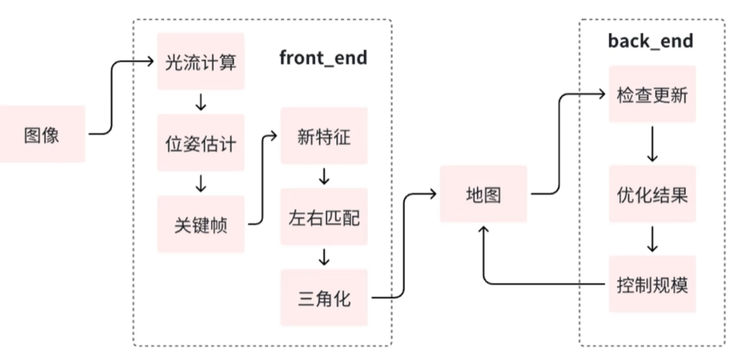
为了提高实践能力，对《SLAM十四讲》第13章的代码进行学习。其实现了前端和后端，但是没有回环检测。因此这篇文章的目标是看懂已有代码并补充回环检测。

1. 代码解析

1.1主函数run_kitti_stereo.cpp

使用了 google::ParseCommandLineFlags(&argc,&argv,ture);处理命令行命令。

DEFINE_string(config_file, "./config/default.yaml", "config file path");
int main(int argc, char **argv) {google::ParseCommandLineFlags(&argc, &argv, true);// 创建视觉里程计对象myslam::VisualOdometry::Ptr vo(new myslam::VisualOdometry(FLAGS_config_file));
...

使用方法：

1. 首先用DEFINE_string定义一个string类型的变量config_file，其默认值是"./config/default.yaml"。参数说明是"config file path"。参数说明让代码阅读者能够快速理解每个参数的作用，提高代码的可维护性。
2. 用google::ParseCommandLineFlags读取命令，ture表示参数读取后从argv中去除。
3. 用FLAGS_config_file使用参数。用法：FLAGS_定义的参数名。

基本流程

int main(int argc, char **argv) {google::ParseCommandLineFlags(&argc, &argv, true);// 1.创建视觉里程计对象，把配置文件地址传入myslam::VisualOdometry::Ptr vo(new myslam::VisualOdometry(FLAGS_config_file));// 2.初始化系统if (!vo->Init()) {std::cerr << "Failed to initialize Visual Odometry!" << std::endl;return -1;}std::cout << "Visual Odometry initialized successfully!" << std::endl;// 3.运行vo->Run();return 0;
}

1. Ptr 是myslam::VisualOdometry类中定义的一个智能指针的类型别名。正常应该写成std::shared_ptr Ptr。在类中定义了typedef std::shared_ptr Ptr;可以简化代码，不用每次写这么长一串。
2. 创建了一个VisualOdometry类的指针变量vo，调用类函数Init初始化，Run运行接下来的流程。

1.1.1bool VisualOdometry::Init()

VisualOdometry类首先在Visual_Odometry.h中定义，然后在Visual_Odometry.cpp中重载。dataset_，frontend_等变脸也是先在Visual_Odometry.h中VisualOdometry类定义的。

bool VisualOdometry::Init() {//用Config类中的SetParameterFile尝试读取配置文档，失败则停止if (Config::SetParameterFile(config_file_path_) == false) {return false;}//创建一个 Dataset 类的智能指针对象，读取配置文件中"dataset_dir"对应的信息//并将其赋值给成员变量 dataset_dataset_ = Dataset::Ptr(new Dataset(Config::Get<std::string>("dataset_dir")));//CHECK_EQ 是一种断言宏（Google 的 glog 或 gtest 库）//它判断括号内的两个表达式是否相等。//如果 dataset_->Init() 的返回值不是 true，程序会立即中断，并输出错误信息。CHECK_EQ(dataset_->Init(), true);//创建各个模块的变量frontend_ = Frontend::Ptr(new Frontend);backend_ = Backend::Ptr(new Backend);map_ = Map::Ptr(new Map);viewer_ = Viewer::Ptr(new Viewer);//设置前端模块的各个调用变量frontend_->SetBackend(backend_);frontend_->SetMap(map_);frontend_->SetViewer(viewer_);frontend_->SetCameras(dataset_->GetCamera(0), dataset_->GetCamera(1));//同理设置后端模块backend_->SetMap(map_);backend_->SetCameras(dataset_->GetCamera(0), dataset_->GetCamera(1));//同理设置可视化模块viewer_->SetMap(map_);return true;
}

1.1.1.1bool Config::SetParameterFile(const std::string &filename)

查看是否存在配置文件，如果有就以只读模式打开，方便后续读取

bool Config::SetParameterFile(const std::string &filename) {if (config_ == nullptr)config_ = std::shared_ptr<Config>(new Config);config_->file_ = cv::FileStorage(filename.c_str(), cv::FileStorage::READ);if (config_->file_.isOpened() == false) {LOG(ERROR) << "parameter file " << filename << " does not exist.";config_->file_.release();return false;}return true;
}

1.1.1.2bool Dataset::Init()

从文件中读取四个相机的投影矩阵参数，并据此初始化相机对象，存储到 cameras_ 容器中

Dataset::Dataset(const std::string& dataset_path): dataset_path_(dataset_path) {}bool Dataset::Init() {ifstream fin(dataset_path_ + "/calib.txt");if (!fin) {LOG(ERROR) << "cannot find " << dataset_path_ << "/calib.txt!";return false;}for (int i = 0; i < 4; ++i) {std::string camera_name;fin >> camera_name; // 直接读取相机名（如P0:）double p[12];for (double &v : p) fin >> v;Mat33 K;K << p[0], p[1], p[2],p[4], p[5], p[6],p[8], p[9], p[10];Vec3 t;t << p[3], p[7], p[11];t = K.inverse() * t;K *= 0.5;cameras_.emplace_back(new Camera(K(0,0), K(1,1), K(0,2), K(1,2), t.norm(), SE3(SO3(), t)));LOG(INFO) << "Camera " << i << " extrinsics: " << t.transpose();}fin.close();current_image_index_ = 0;return true;
}

1.1.2 void VisualOdometry::Run()

循环，直到运行函数Step()输出0

void VisualOdometry::Run() {do {LOG(INFO) << "VO is running";} while (Step());backend_->Stop();viewer_->Close();LOG(INFO) << "VO exit";
}

1.1.2.1 bool VisualOdometry::Step()

bool VisualOdometry::Step() {Frame::Ptr new_frame = dataset_->NextFrame();if (new_frame == nullptr) return false;auto t1 = std::chrono::steady_clock::now();bool success = frontend_->AddFrame(new_frame);auto t2 = std::chrono::steady_clock::now();auto time_used =std::chrono::duration_cast<std::chrono::duration<double>>(t2 - t1);LOG(INFO) << "VO cost time: " << time_used.count() << " seconds.";return success;
}

1.1.2.1.1Frame::Ptr Dataset::NextFrame()

Frame::Ptr Dataset::NextFrame() {boost::format fmt("%s/image_%d/%06d.png");cv::Mat image_left, image_right;// read imagesimage_left =cv::imread((fmt % dataset_path_ % 0 % current_image_index_).str(),cv::IMREAD_GRAYSCALE);image_right =cv::imread((fmt % dataset_path_ % 1 % current_image_index_).str(),cv::IMREAD_GRAYSCALE);if (image_left.data == nullptr || image_right.data == nullptr) {LOG(WARNING) << "cannot find images at index " << current_image_index_;return nullptr;}cv::Mat image_left_resized, image_right_resized;cv::resize(image_left, image_left_resized, cv::Size(), 0.5, 0.5,cv::INTER_NEAREST);cv::resize(image_right, image_right_resized, cv::Size(), 0.5, 0.5,cv::INTER_NEAREST);auto new_frame = Frame::CreateFrame();new_frame->left_img_ = image_left_resized;new_frame->right_img_ = image_right_resized;current_image_index_++;return new_frame;
}

1.1.2.2bool Frontend::AddFrame(myslam::Frame::Ptr frame)

用于处理每一帧新输入的图像数据。

bool Frontend::AddFrame(myslam::Frame::Ptr frame) {current_frame_ = frame;switch (status_) {case FrontendStatus::INITING:StereoInit();break;case FrontendStatus::TRACKING_GOOD:case FrontendStatus::TRACKING_BAD:Track();break;case FrontendStatus::LOST:Reset();break;}last_frame_ = current_frame_;return true;
}

其主要流程如下：
首先，将传入的帧指针 frame 赋值给成员变量 current_frame_，表示当前正在处理的帧。然后，根据前端当前的状态 status_，选择不同的处理逻辑：

1. 如果状态为 INITING（初始化中），调用 StereoInit() 方法进行立体初始化，通常用于系统刚启动时建立初始地图和位姿。
2. 如果状态为 TRACKING_GOOD 或 TRACKING_BAD，说明系统已经初始化并在跟踪状态，此时调用 Track() 方法进行正常的帧间跟踪和位姿估计。
3. 如果状态为 LOST，表示跟踪失败或丢失，调用 Reset() 方法尝试重置系统（当前实现仅输出提示信息）。

无论哪种状态，最后都会将 current_frame_ 赋值给 last_frame_，为下一帧的处理做准备。函数最后返回 true，表示处理流程已完成。

处理当前帧的处理函数：

1. StereoInit()
   实现了视觉前端的立体初始化流程。其主要目的是在系统启动时，通过双目图像建立初始地图和关键帧，为后续的跟踪与建图打下基础。

bool Frontend::StereoInit() {int num_features_left = DetectFeatures();int num_coor_features = FindFeaturesInRight();if (num_coor_features < num_features_init_) {return false;}bool build_map_success = BuildInitMap();if (build_map_success) {status_ = FrontendStatus::TRACKING_GOOD;if (viewer_) {viewer_->AddCurrentFrame(current_frame_);viewer_->UpdateMap();}return true;}return false;
}

首先，函数调用 DetectFeatures() 在当前帧的左图像中检测特征点，并记录检测到的数量。接着，调用 FindFeaturesInRight()，在右图像中寻找与左图像特征点对应的点对，并统计成功匹配的特征数量。

如果找到的左右特征点对数量小于设定的阈值 num_features_init_，说明初始化条件不足，函数直接返回 false，表示初始化失败。

如果特征点对数量充足，函数继续调用 BuildInitMap()，尝试通过三角化建立初始地图点。如果地图构建成功，则将前端状态切换为 TRACKING_GOOD，表示系统已完成初始化并进入正常跟踪状态。此时，如果有可视化模块（viewer_），则更新当前帧和地图的显示。最后返回 true，表示初始化成功。

如果地图构建失败，则返回 false。整个流程体现了初始化阶段的典型步骤：特征检测、特征匹配、三角化建图和状态切换。

2. Track()
   它的核心任务是根据上一帧的信息，对当前帧进行位姿估计和状态判断，并根据跟踪情况维护关键帧和地图。

bool Frontend::Track() {if (last_frame_) {current_frame_->SetPose(relative_motion_ * last_frame_->Pose());}int num_track_last = TrackLastFrame();tracking_inliers_ = EstimateCurrentPose();if (tracking_inliers_ > num_features_tracking_) {// tracking goodstatus_ = FrontendStatus::TRACKING_GOOD;} else if (tracking_inliers_ > num_features_tracking_bad_) {// tracking badstatus_ = FrontendStatus::TRACKING_BAD;} else {// loststatus_ = FrontendStatus::LOST;}InsertKeyframe();relative_motion_ = current_frame_->Pose() * last_frame_->Pose().inverse();if (viewer_) viewer_->AddCurrentFrame(current_frame_);return true;
}

4. Reset()

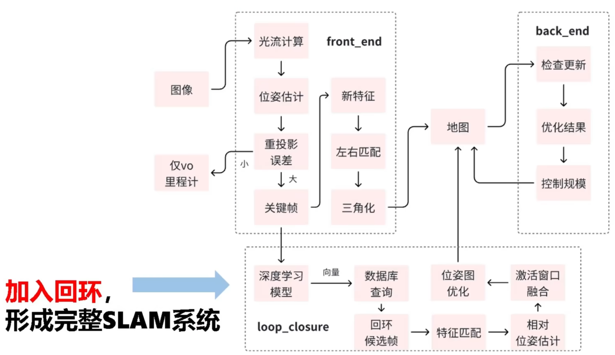
2. 回环检测

前沿的回环检测算法概述

回环检测（Loop Closure Detection）是机器人学、计算机视觉和SLAM（同时定位与地图构建）中的关键技术，用于识别机器人是否返回了之前访问过的位置，从而校正累积误差并优化地图构建。随着深度学习的发展，前沿算法已从传统特征匹配转向数据驱动方法，结合高效的特征提取和相似度计算。以下列出当前主要的前沿算法，每个算法均简要解释其原理和优势。

1. NetVLAD

• 原理：基于卷积神经网络（CNN）和VLAD（Vector of Locally Aggregated Descriptors）编码器，将图像转换为全局描述符。通过端到端训练，学习区分性特征，用于图像检索。
• 优势：鲁棒性强，对光照和视角变化不敏感；计算效率高，适合实时应用。
• 数学基础：相似度计算使用余弦相似度：
  $$s=\frac{\mathbf{f}\cdot \mathbf{g}}{\Vert \mathbf{f}\Vert \cdot \Vert \mathbf{g}\Vert }$$
  其中$\mathbf{f}$和$\mathbf{g}$是特征向量。

2. SeqSLAM

• 原理：考虑图像序列的时空一致性，而非单帧匹配。通过局部对比度归一化处理光照变化，并基于序列窗口进行相似度搜索。
• 优势：在极端环境变化（如季节变换）下表现优异；计算复杂度低。
• 应用场景：常用于自动驾驶和无人机导航。

3. PointNetVLAD

• 原理：专为点云数据设计，结合PointNet（点云特征提取网络）和VLAD编码。将3D点云转换为紧凑描述符，用于回环检测。
• 优势：处理非结构化数据能力强；支持LiDAR和RGB-D传感器。
• 数学基础：特征聚合公式：
  $$\mathbf{v}=\sum _{i=1}^N{\alpha }_i\cdot {\mathbf{f}}_i$$
  其中${\mathbf{f}}_i$是点特征，${\alpha }_i$是注意力权重。

4. OverlapNet

• 原理：利用深度神经网络预测点云之间的重叠区域和相对位姿。融合几何和语义信息（如高度图和法向量）。
• 优势：高精度，减少误检率；适用于大规模环境。
• 趋势：常与图优化方法（如位姿图优化）结合使用。

5. 基于Transformer的模型（如LoopTransformer）

• 原理：采用Transformer架构，处理图像或点云序列的长期依赖关系。通过自注意力机制学习全局上下文。
• 优势：在复杂场景中泛化性好；支持多模态数据融合。
• 示例：相似度得分计算：
  $$s=\text{softmax}\left(\frac{Q{K}^T}{\sqrt{d_k}}\right)V$$
  其中$Q,K,V$是查询、键和值矩阵。

6. DeepLCD

• 原理：端到端深度学习方法，直接从原始数据学习回环检测决策。使用Siamese网络结构比较特征对。
• 优势：减少人工特征工程；适应性强。
• 代码示例：以下是一个简化的PyTorch伪代码，展示特征匹配过程：

  import torch
  import torch.nn as nnclass LoopDetector(nn.Module):def __init__(self):super().__init__()self.cnn = nn.Sequential(  # 特征提取网络nn.Conv2d(3, 64, kernel_size=3),nn.ReLU(),nn.MaxPool2d(2))self.fc = nn.Linear(64 * 14 * 14, 128)  # 特征向量维度128def forward(self, img1, img2):feat1 = self.cnn(img1)feat1 = feat1.view(feat1.size(0), -1)feat1 = self.fc(feat1)feat2 = self.cnn(img2)feat2 = feat2.view(feat2.size(0), -1)feat2 = self.fc(feat2)similarity = torch.cosine_similarity(feat1, feat2, dim=1)  # 余弦相似度return similarity
  

总结与趋势

• 当前前沿：算法正从传统方法（如词袋模型BoW）向深度学习过渡，NetVLAD和Transformer模型成为主流。
• 关键挑战：处理动态环境、计算效率和跨传感器泛化。
• 未来方向：结合强化学习优化决策，以及多模态融合（如视觉-LiDAR）提升鲁棒性。