DIEN:深度兴趣演化网络
实验和完整代码
代码实现和jupyter实验:https://github.com/Myolive-Lin/RecSys--deep-learning-recommendation-system/tree/main
引言
深度兴趣演化网络 (DIEN) 旨在解决在用户意图不明确的情况下(如在线展示广告)进行点击率预测(CTR)的挑战。它通过捕捉和建模用户兴趣及其随时间演化的过程,提升了CTR预测的效果。本文将详细介绍DIEN的架构,重点讲解其核心模块:兴趣提取层和兴趣演化层。
深度兴趣演化网络 (DIEN)
与受控搜索不同,在许多电商平台(如在线展示广告)中,用户的意图并不明显,因此捕捉用户兴趣及其动态变化对CTR预测至关重要。DIEN专注于捕捉用户兴趣并建模兴趣的演化过程。DIEN的架构如下图所示。
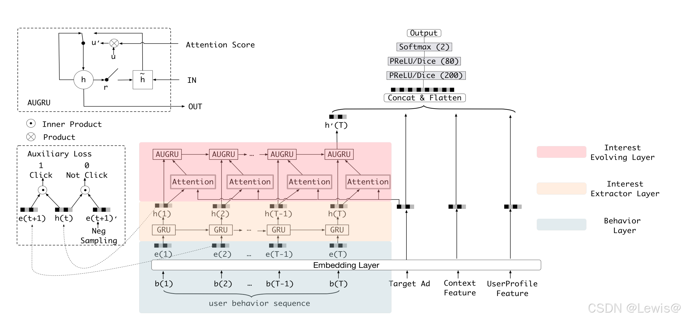
DIEN由以下几个部分组成:
- 所有特征类别通过嵌入层进行转换。
- DIEN采取两步法来捕捉兴趣演化:
- 兴趣提取层:基于用户行为序列提取兴趣序列。
- 兴趣演化层:建模与目标项相关的兴趣演化过程。
- 最终的兴趣表示与广告、用户画像和上下文的嵌入向量进行拼接,拼接后的向量输入多层感知机(MLP)进行最终预测。
兴趣提取层
在电商系统中,用户行为承载着潜在的兴趣,用户在每次行为后,兴趣都会发生变化。在兴趣提取层,作者从用户的行为序列中提取一系列的兴趣状态。
电商系统中的用户点击行为非常丰富,历史行为序列的长度即使在短时间内(例如两周)也非常长。为了在效率与性能之间找到平衡,作者使用GRU(门控循环单元)来建模行为之间的依赖关系,GRU的输入是按时间顺序排列的用户行为。GRU克服了RNN中的梯度消失问题,比LSTM速度更快,适合电商系统。GRU的公式如下:
u t = σ ( W u i t + U u h t − 1 + b u ) u_t = \sigma(W_u i_t + U_u h_{t-1} + b_u) ut=σ(Wuit+Uuht−1+bu)
r t = σ ( W r i t + U r h t − 1 + b r ) r_t = \sigma(W_r i_t + U_r h_{t-1} + b_r) rt=σ(Writ+Urht−1+br)
h ~ t = tanh ( W h i t + r t ∘ U h h t − 1 + b h ) \tilde{h}_t = \tanh(W_h i_t + r_t \circ U_h h_{t-1} + b_h) h~t=tanh(Whit+rt∘Uhht−1+bh)
h t = ( 1 − u t ) ∘ h t − 1 + u t ∘ h ~ t h_t = (1 - u_t) \circ h_{t-1} + u_t \circ \tilde{h}_t ht=(1−ut)∘ht−1+ut∘h~t
其中, σ \sigma σ是Sigmoid激活函数, ∘ \circ ∘表示逐元素乘积, W u , W r , W h ∈ R n H × n I W_u, W_r, W_h \in \mathbb{R}^{n_H \times n_I} Wu,Wr,Wh∈RnH×nI, U z , U r , U h ∈ R n H × n H U_z, U_r, U_h \in \mathbb{R}^{n_H \times n_H} Uz,Ur,Uh∈RnH×nH, n H n_H nH是隐藏层大小, n I n_I nI是输入大小。 i t i_t it是GRU的输入,表示用户在 t t t时刻的行为, h t h_t ht是 t t t时刻的隐藏状态。
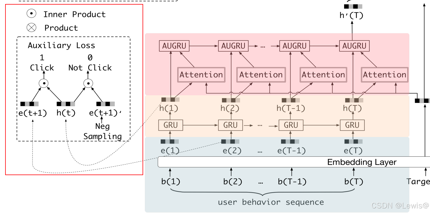
然而,仅仅依赖GRU的隐藏状态 h t h_t ht来捕捉行为之间的依赖关系不足以有效表示兴趣。因此,提出了辅助损失(Auxiliary Loss),它通过使用下一次行为 b t + 1 b_{t+1} bt+1来监督兴趣状态 h t h_t ht的学习。除了使用实际的下一次行为作为正样本外,作者还从非点击项中采样负样本。
辅助损失可以表示为:
L a u x = − 1 N ∑ i = 1 N ∑ t log σ ( h i t , e i b [ t + 1 ] ) + log ( 1 − σ ( h i t , e ^ i b [ t + 1 ] ) ) L_{aux} = -\frac{1}{N} \sum_{i=1}^{N} \sum_{t} \log \sigma(h_i^t, e_i^{b[t+1]}) + \log(1 - \sigma(h_i^t, \hat{e}_i^{b[t+1]})) Laux=−N1i=1∑Nt∑logσ(hit,eib[t+1])+log(1−σ(hit,e^ib[t+1]))
其中, σ ( x 1 , x 2 ) \sigma(x_1, x_2) σ(x1,x2)是Sigmoid激活函数, h i t h_i^t hit表示用户 i i i在 t t t时刻的GRU隐藏状态。最终的全局损失函数为:
L = L t a r g e t + α ⋅ L a u x L = L_{target} + \alpha \cdot L_{aux} L=Ltarget+α⋅Laux
其中,
α
\alpha
α是调节兴趣表示和CTR预测之间平衡的超参数。
损失函数如下:
在深度CTR模型中,广泛使用的损失函数是负对数似然函数(Negative Log-Likelihood),它利用目标项的标签来监督整体预测:
L t a r g e t = − 1 N ∑ ( x , y ) ∈ D ( y log p ( x ) + ( 1 − y ) log ( 1 − p ( x ) ) ) L_{target} = -\frac{1}{N} \sum_{(x,y) \in D} \left( y \log p(x) + (1 - y) \log(1 - p(x)) \right) Ltarget=−N1(x,y)∈D∑(ylogp(x)+(1−y)log(1−p(x)))
其中, x = [ x p , x a , x c , x b ] ∈ D x = [x_p, x_a, x_c, x_b] \in D x=[xp,xa,xc,xb]∈D, D D D是训练集,大小为 N N N, y ∈ { 0 , 1 } y \in \{0, 1\} y∈{0,1}表示用户是否点击目标项, p ( x ) p(x) p(x)是网络输出,表示用户点击目标项的预测概率。
兴趣演化层
用户的兴趣在外部环境和内部认知的共同作用下随时间演化。例如,用户对衣服的兴趣可能会随人口趋势和个人口味的变化而变化。兴趣演化层的目标是通过建模兴趣的演化过程,提高目标项CTR的预测准确度。
在兴趣演化过程中,兴趣表现出两个特征:
- 兴趣漂移:由于兴趣的多样性,兴趣可能会发生漂移。例如,用户在某一段时间内对书籍感兴趣,而在另一段时间内对衣服感兴趣。
- 兴趣之间的相互影响:尽管兴趣之间可能会互相影响,但每种兴趣都有独立的演化过程。作者关注的是与目标项相关的兴趣演化过程。
为了建模兴趣的演化过程,DIEN结合了GRU的顺序学习能力和注意力机制的局部激活能力。具体而言,兴趣演化层通过对每个GRU步骤的局部激活,使得与目标项相关的兴趣得以强化,减少来自兴趣漂移的干扰。
作者提出了几种结合注意力机制和GRU的兴趣演化方法:
- GRU with Attentional Input (AIGRU):通过注意力得分影响兴趣演化输入,但效果较差,因为即使输入为零,也会影响GRU的隐藏状态。
- Attention-based GRU (AGRU):AGRU通过将注意力得分嵌入GRU架构,直接控制隐藏状态的更新,从而更有效地提取与目标项相关的兴趣。
- GRU with Attentional Update Gate (AUGRU):AUGRU结合了注意力机制和GRU的更新门,能够更加精细地控制每个维度的兴趣演化,从而更有效地避免兴趣漂移的干扰。
Attention计算如下
a
t
=
e
x
p
(
h
t
W
e
a
)
∑
j
=
1
T
e
x
p
(
h
j
W
e
a
)
a_t = \frac{exp(h_t We_a)}{\sum_{j=1}^{T} exp(h_jWe_a)}
at=∑j=1Texp(hjWea)exp(htWea)
其中 e a e_a ea 是从类别广告(category ad)中的字段拼接(concat)得到的嵌入向量, W ∈ R n H × n A W ∈ R^{n_H×n_A} W∈RnH×nA,其中 n H n_H nH 是隐藏状态的维度, n A n_A nA 是广告嵌入向量的维度。注意力得分(Attention score)反映了广告 e a e_a ea和输入 h t h_t ht 之间的关系,强关联性会导致较大的注意力得分
以下是具体实现的几种方法
| 方法 | 公式 | 优势 | 局限 |
|---|---|---|---|
| AIGRU | i t ′ = h t ⊙ a t i'_t = h_t \odot a_t it′=ht⊙at | 简单实现 | 零输入仍影响隐状态 |
| AGRU | h t ′ = ( 1 − a t ) h t − 1 ′ + a t h ~ t h'_t = (1-a_t)h'_{t-1} + a_t\tilde{h}_t ht′=(1−at)ht−1′+ath~t | 直接控制隐状态更新 | 标量注意力丢失维度信息 |
| AUGRU | u ~ t = a t ⊙ u t \tilde{u}_t = a_t \odot u_t u~t=at⊙ut | 保持门控维度特性 | 计算复杂度略高 |
| h t ′ = ( 1 − u ~ t ) h t − 1 ′ + u ~ t h ~ t h'_t = (1-\tilde{u}_t)h'_{t-1} + \tilde{u}_t\tilde{h}_t ht′=(1−u~t)ht−1′+u~th~t | 精准调节兴趣演化轨迹 |
代码实现
官方代码
torch实现如下
GRU单元
class GRUCell(nn.Module):
    def __init__(self, input_dim, hidden_dim):
        super(GRUCell, self).__init__()
        self.input_dim = input_dim
        self.hidden_dim = hidden_dim

        # Update Gate
        self.Wu = nn.Linear(input_dim, hidden_dim, bias=True)
        self.Uu = nn.Linear(hidden_dim, hidden_dim, bias=False)

        # Reset Gate
        self.Wr = nn.Linear(input_dim, hidden_dim, bias=True)
        self.Ur = nn.Linear(hidden_dim, hidden_dim, bias=False)

        # Candidate Hidden State
        self.Wh = nn.Linear(input_dim, hidden_dim, bias=True)
        self.Uh = nn.Linear(hidden_dim, hidden_dim, bias=False)

    def forward(self, x, h_prev):
        """
        Forward pass of the GRU cell.
        Args:
            x: Input at current time step (batch_size, input_dim).
            h_prev: Previous hidden state (batch_size, hidden_dim).
        Returns:
            h_next: Next hidden state (batch_size, hidden_dim).
        """
        u = torch.sigmoid(self.Wu(x) + self.Uu(h_prev))  # Update gate
        r = torch.sigmoid(self.Wr(x) + self.Ur(h_prev))  # Reset gate
        h_tilde = torch.tanh(self.Wh(x) + r * self.Uh(h_prev))  # Candidate hidden state
        h_next = (1 - u) * h_prev + u * h_tilde  # Final hidden state

        return h_next
Interest Extractor Layer 兴趣提取层
class InterestExtractor(nn.Module):
    def __init__(self, input_dim, hidden_dim):
        super(InterestExtractor, self).__init__()
        self.gru_cell = GRUCell(input_dim, hidden_dim)

    def forward(self, x):
        """
        Forward pass of the Interest Extractor Layer.
        Args:
            x: Behavior sequence (batch_size, seq_len, input_dim).
        Returns:
            hidden_states: Hidden states of GRU (batch_size, seq_len, hidden_dim).
        """

        batch_size, seq_len, _ = x.size()
        hidden_states = []
        h_t =  torch.zeros(batch_size, self.gru_cell.hidden_dim, device = x.device ) #(batch_size, hidden_dim)

        for t in range(seq_len):
            h_t = self.gru_cell(x[: , t, :],h_t)
            hidden_states.append(h_t)

        hidden_states = torch.stack(hidden_states, dim = 1) # (batch_size, seq_len, hidden_dim)

        return hidden_states
AUGRU 单元
#其实就是在u的部分加入Attention得分计算h_t
class AUGRUCell(nn.Module):
    def __init__(self, input_dim, hidden_dim):
        super(AUGRUCell, self).__init__()
        self.input_dim = input_dim
        self.hidden_dim = hidden_dim

        #Update gate
        self.Wu = nn.Linear(input_dim, hidden_dim, bias = True)
        self.Uu = nn.Linear(hidden_dim, hidden_dim, bias = False)

        #Rest Gate
        self.Wr = nn.Linear(input_dim, hidden_dim, bias = True)
        self.Ur = nn.Linear(hidden_dim, hidden_dim, bias= False)

        #Candidate Hidden State
        self.Wh = nn.Linear(input_dim, hidden_dim, bias= True)
        self.Uh = nn.Linear(hidden_dim, hidden_dim, bias= False)

        #注意力权重矩阵
        self.attention_weight = nn.Parameter(torch.randn(input_dim , input_dim)) # W ∈ R^(nH × nA) , nH是输入维度,nA是输入的target的纬度

    def __init__weights(self):
        for name, param in self.named_parameters():
            if 'W_a' in name:
                nn.init.xavier_normal_(param)
            if 'W_' in name or 'U_'in name:
                nn.init.orthogonal_(param)

    def forward(self, hidden_states, target_embd):
        """
        hidden_states: [B, T, D]
        target_emb: [B, D]
        """
        batch_size, seq_lens,_  = hidden_states.size()

        #计算注意力得分
        target_expanded = target_embd.unsqueeze(1) #[B, 1, D]
        hidden_states_mapped = torch.matmul(hidden_states, self.attention_weight) #[B,T,D]
        att_input = torch.matmul(hidden_states_mapped, target_expanded.transpose(1,2)) #[B,T,1]
        att_input = att_input.squeeze(-1) # [B, T],去掉多余的维度
        attention_scores = F.softmax(att_input, dim = 1).unsqueeze(-1) # [B, T] - > # [B, T,1]

        # AUGRU处理 ----------------------------------------------------
        h_t = torch.zeros(batch_size, self.hidden_dim, device = hidden_states.device)

        for t in range(seq_lens):
            att_t = attention_scores[:, t, :] # [B, 1]

            #当前隐藏状态
            x_t = hidden_states[:, t, :] # [B, D]

            #更新门 (加入注意力权重)
            u = torch.sigmoid(self.Wu(x_t) + self.Uu(h_t)) * att_t

            #重置门
            r = torch.sigmoid(self.Wr(x_t) + self.Ur(h_t))

            #候选状态
            h_tilde = torch.tanh(self.Wh(x_t)  + self.Uh(h_t))

            #更新隐藏状态
            h_t = (1 - u) * h_t + u * h_tilde

        return h_t #返回最后的兴趣
Dice 激活函数
这部分和DIN一样,具体公式不再展开
class Dice(nn.Module):
    def __init__(self, alpha=0.0, epsilon=1e-8):
        """
        初始化 Dice 激活函数。
        :param alpha: 可学习的参数,用于控制负值部分的缩放。
        :param epsilon: 一个小常数,用于数值稳定性。
        """
        super(Dice, self).__init__()
        self.alpha = nn.Parameter(torch.tensor(alpha))  # 可学习参数
        self.epsilon = epsilon

    def forward(self, x):
        """
        前向传播函数。
        :param x: 输入张量,形状为 (batch_size, ...)。
        :return: 经过 Dice 激活后的张量。
        """
        # 计算输入 x 的均值和方差
        mean = x.mean(dim=0, keepdim=True)  # 沿 batch 维度计算均值,保留维度
        var = x.var(dim=0, keepdim=True, unbiased=False)  # 沿 batch 维度计算方差,不使用无偏估计

        # 计算控制函数 p(s)
        p_s = 1 / (1 + torch.exp(-(x - mean) / torch.sqrt(var + self.epsilon)))

        # 应用 Dice 激活函数
        output = p_s * x + (1 - p_s) * self.alpha * x
        return output
DIEN模型构建
class DIEN(nn.Module):
    def __init__(self, user_num, item_num, cate_num, emb_dim=18, hidden_dim= [200, 80]):
        super(DIEN, self).__init__()
        self.emb_dim = emb_dim
        self.hidden_dim = hidden_dim

        #嵌入层
        self.user_embedding = nn.Embedding(user_num, emb_dim)
        self.item_embedding = nn.Embedding(item_num, emb_dim)
        self.cate_embedding = nn.Embedding(cate_num, emb_dim)

        #兴趣提取层吗,为了简介,兴趣提取层和兴趣演化层的不做维度改变
        self.interest_extractor = InterestExtractor(input_dim = emb_dim *2, hidden_dim = emb_dim *2,)  #注意这里是emb_dim * 2 因为输入数据是item_id 和 cate_id 的拼接,且不做维度变化

        #兴趣演化层
        self.evolution = AUGRUCell(input_dim = emb_dim * 2, hidden_dim = emb_dim*2 ) #由于输入数据是原本的item_id 和 cate_id 的拼接 所以维度要*2

        self.final_dim = emb_dim * 4 + emb_dim #最后一个是h'(T)即是兴趣演化层输出长度
        #预测层
        fc = []
        for hid_dim in hidden_dim:
            fc.append(nn.Linear(self.final_dim, hid_dim))
            fc.append(Dice()) #使用Dice激活函数
            self.final_dim = hid_dim
        fc.append(nn.Linear(hidden_dim[-1], 2))
        self.fc = nn.Sequential(*fc)

    def forward(self,user_id, target_item, target_cate, hist_items, hist_cates):
        """
        user_id: [B]
        target_item: [B]
        target_cate: [B]
        hist_items: [B, T]
        hist_cates: [B, T]
        """

        #嵌入层
        user_embd = self.user_embedding(user_id)

        target_item_emb = self.item_embedding(target_item)
        target_cate_emb = self.cate_embedding(target_cate)
        target_emb = torch.cat([target_item_emb, target_cate_emb], dim=1)

        #处理历史数据
        hist_cates_embd = self.cate_embedding(hist_cates)
        hist_items_embd = self.item_embedding(hist_items)
        hist_emb  = torch.cat([hist_items_embd, hist_cates_embd], dim=-1)

        # 兴趣提取
        hidden_states = self.interest_extractor(hist_emb)

        # 兴趣演化
        h_t = self.evolution(hidden_states, target_emb) # 与target_emb 计算出最后的h'(T)

        #最终预测
        final_emb = torch.cat([user_embd, target_emb, h_t], dim = 1)
        output = self.fc(final_emb)
        return torch.softmax(output, dim = 1), hidden_states # hidden_states 是为了方面便后计算 Auxiliary loss
辅助损失函数Auxiliary loss和 DIEN Loss
#loss 函数
class AuxiliaryNet(nn.Module):
    def __init__(self, input_dim):
        super(AuxiliaryNet, self).__init__()
        # 定义网络层
        self.bn1 = nn.BatchNorm1d(input_dim)  # batch normalization
        self.dnn1 = nn.Linear(input_dim, 100)  # 第一个全连接层
        self.dnn2 = nn.Linear(100, 50)  # 第二个全连接层
        self.dnn3 = nn.Linear(50, 2)  # 第三个全连接层,输出两个值用于softmax

    def forward(self, x):
        x = self.bn1(x)
        x = F.sigmoid(self.dnn1(x))
        x = F.sigmoid(self.dnn2(x))
        x = self.dnn3(x)
        return F.softmax(x, dim=-1) + 0.00000001


def dien_loss(ctr_pred, interest_item_emb, labels, hist_items, item_emb, hist_cate, cate_emb ,criterion, alpha = 0.5):
    """
        计算 DIEN 模型的损失函数。
        :param ctr_pred: 预测的点击率,形状为 (batch_size,)。
        :param interest_item_emb: 形状为 (batch_size, max_len, emb_dim)。
        :param labels: 真实标签,形状为 (batch_size,)。
        :param hist_items: 历史物品序列,形状为 (batch_size, max_len)。
        :param item_emb: 物品嵌入层,用于获取物品嵌入。
        :param hist_cate: 历史类别序列,形状为 (batch_size, max_len)。
        :param cate_emb: 类别嵌入层,用于获取类别嵌入。
        :param alpha: 主损失和辅助损失的权重。
        :return: 总损失。
    """
    #mask
    mask = (hist_items != 0).float() #[B, T]

    #主损失
    nn.BCELoss
    main_loss = criterion(ctr_pred, labels)
    main_loss = (main_loss * mask).mean()

    #辅助损失计算
    batch_size, max_len = hist_items.size()

    #正样本: 下一个物品
    pos_items = hist_items[:, 1:].reshape(-1) #[B * (T-1)]
    pos_emb = item_emb(pos_items)             #[B * (T-1), D]

    #正样本: 下一个类别
    pos_cate = hist_cate[:, 1:].reshape(-1) #[B * (T-1)]
    pos_cate_emb = cate_emb(pos_cate)         #[B * (T-1), D]

    pos = torch.cat([pos_emb, pos_cate_emb], dim = 1) #[B * (T-1), 2D]


    #负样本: 从整个物品表随机采样, 但要确保负样本不在用户历史行为序列中
    neg_items = []
    for i in range(batch_size):
        user_hist = hist_items[i, :].tolist()
        user_neg_items = []
        while len(user_neg_items) < (max_len -1):
            neg_item = torch.randint(1, item_emb.num_embeddings, (1,), device = hist_items.device)

            if neg_item not in user_hist:
                user_neg_items.append(neg_item)

        neg_items.append(torch.tensor(user_neg_items, device = hist_items.device)) #[T-1]

    neg_items = torch.cat(neg_items, dim = 0) #[B * (T-1)]
    neg_emb = item_emb(neg_items)             #[B * (T-1), D]

    #负样本: 从整个类别表随机采样, 但要确保负样本不在用户历史行为序列中
    neg_cates = []
    for i in range(batch_size):
        user_hist = hist_cate[i, :].tolist()
        user_neg_cate = []
        while len(user_neg_cate) < (max_len -1):
            neg_cate = torch.randint(1, cate_emb.num_embeddings, (1,), device = hist_cate.device)

            if neg_cate not in user_hist:
                user_neg_cate.append(neg_cate)

        neg_cates.append(torch.tensor(user_neg_cate, device = hist_cate.device)) #[T-1]
    neg_cates = torch.cat(neg_cates, dim = 0) #[B * (T-1)]
    neg_cate_emb = cate_emb(neg_cates)         #[B * (T-1), D]
    neg = torch.cat([neg_emb, neg_cate_emb], dim = 1) #[B * (T-1), 2D]


    # 辅助预测
    h = interest_item_emb[:, :-1, :].reshape(-1, interest_item_emb.size(-1)) # [B * (T-1), D]

    #正负样本计算
    pos_sim = torch.cat([h, pos], dim = 1) #[B * (T-1), 2D]
    neg_sim = torch.cat([h, pos], dim = 1) #[B * (T-1), 2D]

    aux_net = AuxiliaryNet(input_dim = pos_sim.size(1))
    click_prop_ = aux_net(pos_sim) #[B * (T-1), 2]
    noclick_prop_ = aux_net(neg_sim)#[B * (T-1), 2]

    #修改mask维度,以适应后续计算
    mask = mask[:, :-1].reshape(-1)  # Reshaping mask to [B*(T-1),]

    #损失计算
    click_loss = -torch.log(click_prop_[:, 1]) * mask
    nonclick_loss = -torch.log(1 - noclick_prop_[:, 1]) * mask
    aux_loss = torch.mean(click_loss + nonclick_loss)

    return main_loss + alpha * aux_loss
实验
这里使用官方DIEN中local_train_splitByUser提取出来了的数据集,由于数据集过大,仅使用前89999个样本数据地址
| label | userID | itemID | cateID | hist_item_list | hist_cate_list |
|---|---|---|---|---|---|
| 0 | AZPJ9LUT0FEPY | B00AMNNTIA | Literature & Fiction | [0307744434, 0062248391, 0470530707, 097892462…] | [Books, Books, Books, Books, Books] |
| 1 | AZPJ9LUT0FEPY | 0800731603 | Books | [0307744434, 0062248391, 0470530707, 097892462…] | [Books, Books, Books, Books, Books] |
| 0 | A2NRV79GKAU726 | B003NNV10O | Russian | [0814472869, 0071462074, 1583942300, 081253836…] | [Books, Books, Books, Books, Baking, Books, Books, Books] |
| 1 | A2NRV79GKAU726 | B000UWJ91O | Books | [0814472869, 0071462074, 1583942300, 081253836…] | [Books, Books, Books, Books, Baking, Books, Books, Books] |
| 0 | A2GEQVDX2LL4V3 | 0321334094 | Books | [0743596870, 0374280991, 1439140634, 0976475731] | [Books, Books, Books, Books] |
| … | … | … | … | … | … |
| 0 | A3CV7NJJC20JTB | 098488789X | Books | [034545197X, 0765326396, 1605420832, 1451648448] | [Books, Books, Books, Books] |
| 1 | A3CV7NJJC20JTB | 0307381277 | Books | [034545197X, 0765326396, 1605420832, 1451648448] | [Books, Books, Books, Books] |
| 0 | A208PSIK2APSKN | 0957496184 | Books | [0515140791, 147674355X, B0055ECOUA, B007JE1B1…] | [Books, Books, Bibles, Literature & Fiction, Literature & Fiction] |
| 1 | A208PSIK2APSKN | 1480198854 | Books | [0515140791, 147674355X, B0055ECOUA, B007JE1B1…] | [Books, Books, Bibles, Literature & Fiction, Literature & Fiction] |
| 0 | A1GRLKG8JA19OA | B0095VGR4I | Literature & Fiction | [031612091X, 0399163832, 1442358238, 1118017447] | [Books, Books, Books, Books] |
使用Ordinal Encoding处理后得到下面数据集,然后使用Ordinal_itemID,Ordinal_cateID经过Embedding后拼接成的向量来表示目标向量
| label | Ordinal_userID | Ordinal_itemID | Ordinal_cateID | Ordinal_hist_item_list | Ordinal_hist_cate_list |
|---|---|---|---|---|---|
| 0 | 44917 | 68074 | 419 | [206424, 142847, 182786, 69605, 197011] | [386, 386, 386, 386, 386] |
| 1 | 44917 | 101880 | 386 | [206424, 142847, 182786, 69605, 197011] | [386, 386, 386, 386, 386] |
| 0 | 19804 | 6163 | 264 | [78315, 2890, 54255, 137135, 124338] | [386, 386, 300, 386, 386] |
| 1 | 19804 | 21400 | 386 | [78315, 2890, 54255, 137135, 124338] | [386, 386, 300, 386, 386] |
| 0 | 17385 | 220405 | 386 | [0, 30271, 97772, 12556, 137554] | [0, 386, 386, 386, 386] |
| … | … | … | … | … | … |
| 0 | 28177 | 210244 | 386 | [0, 98594, 185606, 19190, 15365] | [0, 386, 386, 386, 386] |
| 1 | 28177 | 16915 | 386 | [0, 98594, 185606, 19190, 15365] | [0, 386, 386, 386, 386] |
| 0 | 12193 | 23175 | 386 | [24471, 189598, 130748, 33111, 100134] | [386, 386, 365, 419, 419] |
| 1 | 12193 | 114216 | 386 | [24471, 189598, 130748, 33111, 100134] | [386, 386, 365, 419, 419] |
| 0 | 5675 | 32074 | 419 | [0, 18220, 48157, 191849, 146917] | [0, 386, 386, 386, 386] |
得到结果如下,模型大概在第2个epoch的时候就已经收敛

Reference
1.王喆《深度学习推荐系统》
2.Zhou, G., Mou, N., Fan, Y., Pi, Q., Bian, W., Zhou, C., Zhu, X., & Gai, K. (Year). Deep Interest Evolution Network for Click-Through Rate Prediction. Alibaba Inc, Beijing, China.
结论
DIEN通过引入兴趣提取层和兴趣演化层,能够有效捕捉用户兴趣并建模其随时间的演化过程。这些创新的模块大大提高了CTR预测的准确性,特别是在用户意图不明确的场景中。通过辅助损失和改进的GRU架构,DIEN能够更好地处理长序列行为数据,并优化用户兴趣的表示,推动广告推荐系统的发展。