python打卡训练营打卡记录day46

知识点回顾：

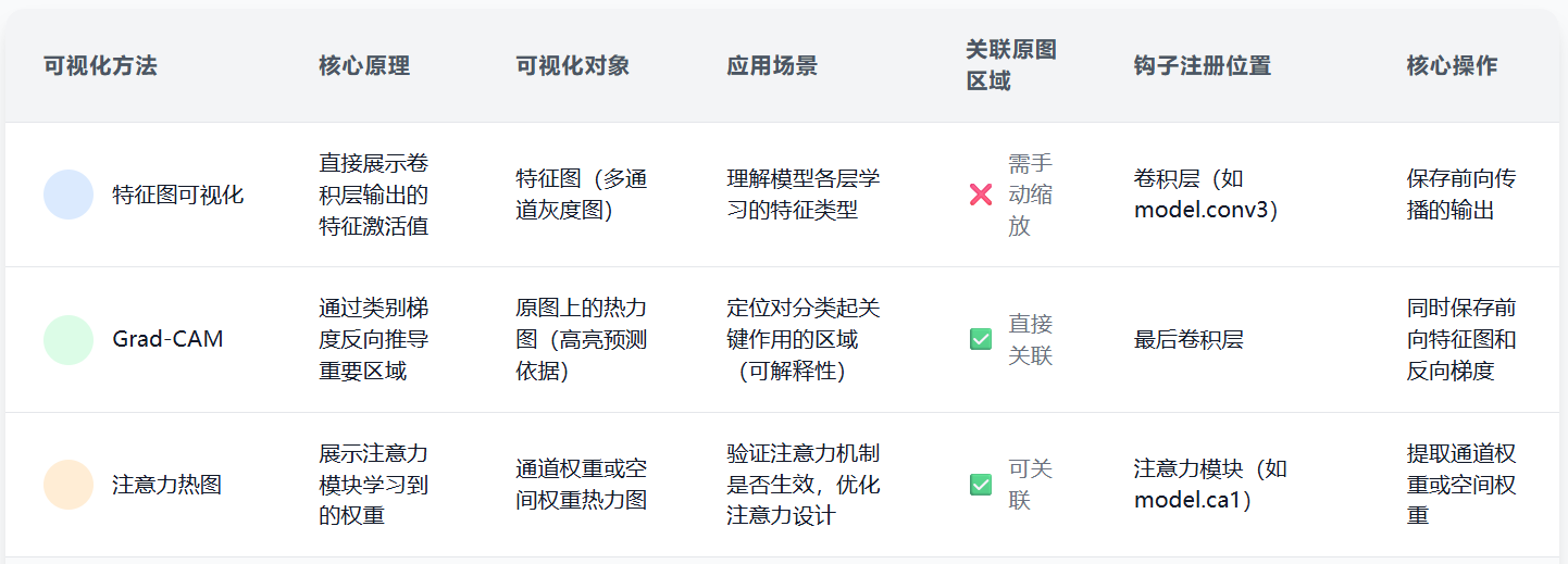
1. 不同CNN层的特征图：不同通道的特征图
2. 什么是注意力：注意力家族，类似于动物园，都是不同的模块，好不好试了才知道。
3. 通道注意力：模型的定义和插入的位置
4. 通道注意力后的特征图和热力图

作业：

1. 今日代码较多，理解逻辑即可
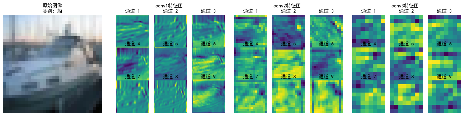
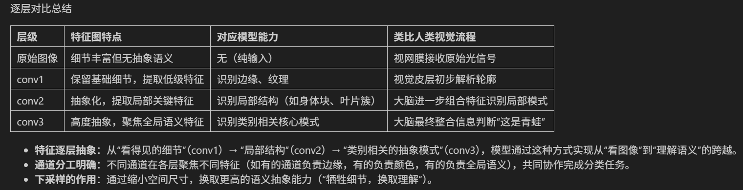
2. 对比不同卷积层特征图可视化的结果（可选）

特征图的提取

CNN训练

import torch
import torch.nn as nn
import torch.optim as optim
from torchvision import datasets, transforms
from torch.utils.data import DataLoader
import matplotlib.pyplot as plt
import numpy as np# 设置中文字体支持
plt.rcParams["font.family"] = ["SimHei"]
plt.rcParams['axes.unicode_minus'] = False  # 解决负号显示问题# 检查GPU是否可用
device = torch.device("cuda" if torch.cuda.is_available() else "cpu")
print(f"使用设备: {device}")# 1. 数据预处理
# 训练集：使用多种数据增强方法提高模型泛化能力
train_transform = transforms.Compose([# 随机裁剪图像，从原图中随机截取32x32大小的区域transforms.RandomCrop(32, padding=4),# 随机水平翻转图像（概率0.5）transforms.RandomHorizontalFlip(),# 随机颜色抖动：亮度、对比度、饱和度和色调随机变化transforms.ColorJitter(brightness=0.2, contrast=0.2, saturation=0.2, hue=0.1),# 随机旋转图像（最大角度15度）transforms.RandomRotation(15),# 将PIL图像或numpy数组转换为张量transforms.ToTensor(),# 标准化处理：每个通道的均值和标准差，使数据分布更合理transforms.Normalize((0.4914, 0.4822, 0.4465), (0.2023, 0.1994, 0.2010))
])# 测试集：仅进行必要的标准化，保持数据原始特性，标准化不损失数据信息，可还原
test_transform = transforms.Compose([transforms.ToTensor(),transforms.Normalize((0.4914, 0.4822, 0.4465), (0.2023, 0.1994, 0.2010))
])# 2. 加载CIFAR-10数据集
train_dataset = datasets.CIFAR10(root='./data',train=True,download=True,transform=train_transform  # 使用增强后的预处理
)test_dataset = datasets.CIFAR10(root='./data',train=False,transform=test_transform  # 测试集不使用增强
)# 3. 创建数据加载器
batch_size = 64
train_loader = DataLoader(train_dataset, batch_size=batch_size, shuffle=True)
test_loader = DataLoader(test_dataset, batch_size=batch_size, shuffle=False)
# 4. 定义CNN模型的定义（替代原MLP）
class CNN(nn.Module):def __init__(self):super(CNN, self).__init__()  # 继承父类初始化# ---------------------- 第一个卷积块 ----------------------# 卷积层1：输入3通道（RGB），输出32个特征图，卷积核3x3，边缘填充1像素self.conv1 = nn.Conv2d(in_channels=3,       # 输入通道数（图像的RGB通道）out_channels=32,     # 输出通道数（生成32个新特征图）kernel_size=3,       # 卷积核尺寸（3x3像素）padding=1            # 边缘填充1像素，保持输出尺寸与输入相同)# 批量归一化层：对32个输出通道进行归一化，加速训练self.bn1 = nn.BatchNorm2d(num_features=32)# ReLU激活函数：引入非线性，公式：max(0, x)self.relu1 = nn.ReLU()# 最大池化层：窗口2x2，步长2，特征图尺寸减半（32x32→16x16）self.pool1 = nn.MaxPool2d(kernel_size=2, stride=2)  # stride默认等于kernel_size# ---------------------- 第二个卷积块 ----------------------# 卷积层2：输入32通道（来自conv1的输出），输出64通道self.conv2 = nn.Conv2d(in_channels=32,      # 输入通道数（前一层的输出通道数）out_channels=64,     # 输出通道数（特征图数量翻倍）kernel_size=3,       # 卷积核尺寸不变padding=1            # 保持尺寸：16x16→16x16（卷积后）→8x8（池化后）)self.bn2 = nn.BatchNorm2d(num_features=64)self.relu2 = nn.ReLU()self.pool2 = nn.MaxPool2d(kernel_size=2)  # 尺寸减半：16x16→8x8# ---------------------- 第三个卷积块 ----------------------# 卷积层3：输入64通道，输出128通道self.conv3 = nn.Conv2d(in_channels=64,      # 输入通道数（前一层的输出通道数）out_channels=128,    # 输出通道数（特征图数量再次翻倍）kernel_size=3,padding=1            # 保持尺寸：8x8→8x8（卷积后）→4x4（池化后）)self.bn3 = nn.BatchNorm2d(num_features=128)self.relu3 = nn.ReLU()  # 复用激活函数对象（节省内存）self.pool3 = nn.MaxPool2d(kernel_size=2)  # 尺寸减半：8x8→4x4# ---------------------- 全连接层（分类器） ----------------------# 计算展平后的特征维度：128通道 × 4x4尺寸 = 128×16=2048维self.fc1 = nn.Linear(in_features=128 * 4 * 4,  # 输入维度（卷积层输出的特征数）out_features=512          # 输出维度（隐藏层神经元数）)# Dropout层：训练时随机丢弃50%神经元，防止过拟合self.dropout = nn.Dropout(p=0.5)# 输出层：将512维特征映射到10个类别（CIFAR-10的类别数）self.fc2 = nn.Linear(in_features=512, out_features=10)def forward(self, x):# 输入尺寸：[batch_size, 3, 32, 32]（batch_size=批量大小，3=通道数，32x32=图像尺寸）# ---------- 卷积块1处理 ----------x = self.conv1(x)       # 卷积后尺寸：[batch_size, 32, 32, 32]（padding=1保持尺寸）x = self.bn1(x)         # 批量归一化，不改变尺寸x = self.relu1(x)       # 激活函数，不改变尺寸x = self.pool1(x)       # 池化后尺寸：[batch_size, 32, 16, 16]（32→16是因为池化窗口2x2）# ---------- 卷积块2处理 ----------x = self.conv2(x)       # 卷积后尺寸：[batch_size, 64, 16, 16]（padding=1保持尺寸）x = self.bn2(x)x = self.relu2(x)x = self.pool2(x)       # 池化后尺寸：[batch_size, 64, 8, 8]# ---------- 卷积块3处理 ----------x = self.conv3(x)       # 卷积后尺寸：[batch_size, 128, 8, 8]（padding=1保持尺寸）x = self.bn3(x)x = self.relu3(x)x = self.pool3(x)       # 池化后尺寸：[batch_size, 128, 4, 4]# ---------- 展平与全连接层 ----------# 将多维特征图展平为一维向量：[batch_size, 128*4*4] = [batch_size, 2048]x = x.view(-1, 128 * 4 * 4)  # -1自动计算批量维度，保持批量大小不变x = self.fc1(x)           # 全连接层：2048→512，尺寸变为[batch_size, 512]x = self.relu3(x)         # 激活函数（复用relu3，与卷积块3共用）x = self.dropout(x)       # Dropout随机丢弃神经元，不改变尺寸x = self.fc2(x)           # 全连接层：512→10，尺寸变为[batch_size, 10]（未激活，直接输出logits）return x  # 输出未经过Softmax的logits，适用于交叉熵损失函数# 初始化模型
model = CNN()
model = model.to(device)  # 将模型移至GPU（如果可用）criterion = nn.CrossEntropyLoss()  # 交叉熵损失函数
optimizer = optim.Adam(model.parameters(), lr=0.001)  # Adam优化器# 引入学习率调度器，在训练过程中动态调整学习率--训练初期使用较大的 LR 快速降低损失，训练后期使用较小的 LR 更精细地逼近全局最优解。
# 在每个 epoch 结束后，需要手动调用调度器来更新学习率，可以在训练过程中调用 scheduler.step()
scheduler = optim.lr_scheduler.ReduceLROnPlateau(optimizer,        # 指定要控制的优化器（这里是Adam）mode='min',       # 监测的指标是"最小化"（如损失函数）patience=3,       # 如果连续3个epoch指标没有改善，才降低LRfactor=0.5        # 降低LR的比例（新LR = 旧LR × 0.5）
)
# 5. 训练模型（记录每个 iteration 的损失）
def train(model, train_loader, test_loader, criterion, optimizer, scheduler, device, epochs):model.train()  # 设置为训练模式# 记录每个 iteration 的损失all_iter_losses = []  # 存储所有 batch 的损失iter_indices = []     # 存储 iteration 序号# 记录每个 epoch 的准确率和损失train_acc_history = []test_acc_history = []train_loss_history = []test_loss_history = []for epoch in range(epochs):running_loss = 0.0correct = 0total = 0for batch_idx, (data, target) in enumerate(train_loader):data, target = data.to(device), target.to(device)  # 移至GPUoptimizer.zero_grad()  # 梯度清零output = model(data)  # 前向传播loss = criterion(output, target)  # 计算损失loss.backward()  # 反向传播optimizer.step()  # 更新参数# 记录当前 iteration 的损失iter_loss = loss.item()all_iter_losses.append(iter_loss)iter_indices.append(epoch * len(train_loader) + batch_idx + 1)# 统计准确率和损失running_loss += iter_loss_, predicted = output.max(1)total += target.size(0)correct += predicted.eq(target).sum().item()# 每100个批次打印一次训练信息if (batch_idx + 1) % 100 == 0:print(f'Epoch: {epoch+1}/{epochs} | Batch: {batch_idx+1}/{len(train_loader)} 'f'| 单Batch损失: {iter_loss:.4f} | 累计平均损失: {running_loss/(batch_idx+1):.4f}')# 计算当前epoch的平均训练损失和准确率epoch_train_loss = running_loss / len(train_loader)epoch_train_acc = 100. * correct / totaltrain_acc_history.append(epoch_train_acc)train_loss_history.append(epoch_train_loss)# 测试阶段model.eval()  # 设置为评估模式test_loss = 0correct_test = 0total_test = 0with torch.no_grad():for data, target in test_loader:data, target = data.to(device), target.to(device)output = model(data)test_loss += criterion(output, target).item()_, predicted = output.max(1)total_test += target.size(0)correct_test += predicted.eq(target).sum().item()epoch_test_loss = test_loss / len(test_loader)epoch_test_acc = 100. * correct_test / total_testtest_acc_history.append(epoch_test_acc)test_loss_history.append(epoch_test_loss)# 更新学习率调度器scheduler.step(epoch_test_loss)print(f'Epoch {epoch+1}/{epochs} 完成 | 训练准确率: {epoch_train_acc:.2f}% | 测试准确率: {epoch_test_acc:.2f}%')# 绘制所有 iteration 的损失曲线plot_iter_losses(all_iter_losses, iter_indices)# 绘制每个 epoch 的准确率和损失曲线plot_epoch_metrics(train_acc_history, test_acc_history, train_loss_history, test_loss_history)return epoch_test_acc  # 返回最终测试准确率# 6. 绘制每个 iteration 的损失曲线
def plot_iter_losses(losses, indices):plt.figure(figsize=(10, 4))plt.plot(indices, losses, 'b-', alpha=0.7, label='Iteration Loss')plt.xlabel('Iteration（Batch序号）')plt.ylabel('损失值')plt.title('每个 Iteration 的训练损失')plt.legend()plt.grid(True)plt.tight_layout()plt.show()# 7. 绘制每个 epoch 的准确率和损失曲线
def plot_epoch_metrics(train_acc, test_acc, train_loss, test_loss):epochs = range(1, len(train_acc) + 1)plt.figure(figsize=(12, 4))# 绘制准确率曲线plt.subplot(1, 2, 1)plt.plot(epochs, train_acc, 'b-', label='训练准确率')plt.plot(epochs, test_acc, 'r-', label='测试准确率')plt.xlabel('Epoch')plt.ylabel('准确率 (%)')plt.title('训练和测试准确率')plt.legend()plt.grid(True)# 绘制损失曲线plt.subplot(1, 2, 2)plt.plot(epochs, train_loss, 'b-', label='训练损失')plt.plot(epochs, test_loss, 'r-', label='测试损失')plt.xlabel('Epoch')plt.ylabel('损失值')plt.title('训练和测试损失')plt.legend()plt.grid(True)plt.tight_layout()plt.show()# 8. 执行训练和测试
epochs = 50  # 增加训练轮次为了确保收敛
print("开始使用CNN训练模型...")
final_accuracy = train(model, train_loader, test_loader, criterion, optimizer, scheduler, device, epochs)
print(f"训练完成！最终测试准确率: {final_accuracy:.2f}%")# # 保存模型
# torch.save(model.state_dict(), 'cifar10_cnn_model.pth')
# print("模型已保存为: cifar10_cnn_model.pth")

特征图可视化

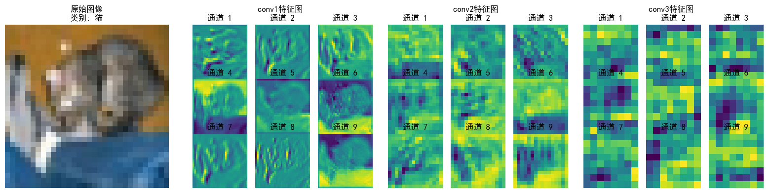
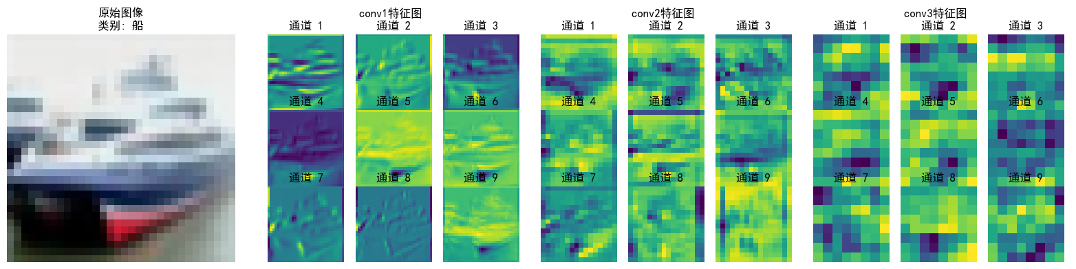
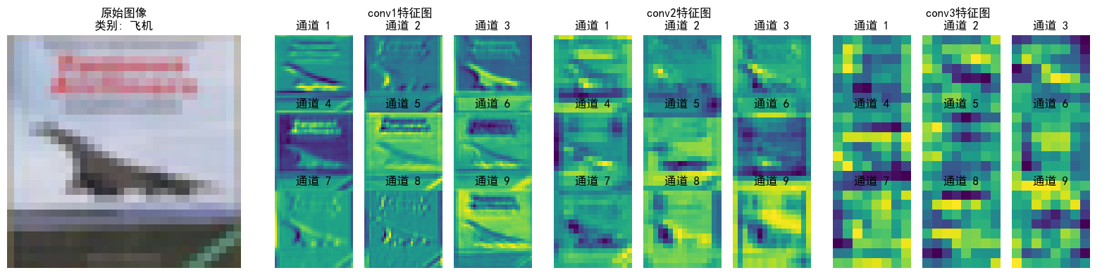
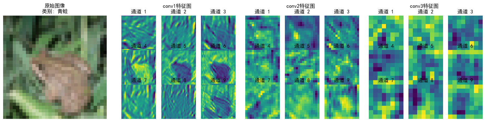
为了方便观察，我们先尝试提取下特征图。特征图本质就是不同的卷积核的输出，浅层指的是离输入图近的卷积层，浅层卷积层的特征图通常较大，而深层特征图会经过多次下采样，尺寸显著缩小，尺寸差异过大时，小尺寸特征图在视觉上会显得模糊或丢失细节。步骤逻辑如下：

1. 初始化设置：
   - 将模型设为评估模式，准备类别名称列表（如飞机、汽车等）。

2. 数据加载与处理：
   - 从测试数据加载器中获取图像和标签。
   - 仅处理前 `num_images` 张图像（如2张）。

3. 注册钩子捕获特征图：
   - 为指定层（如 `conv1`, `conv2`, `conv3`）注册前向钩子。
   - 钩子函数将这些层的输出（特征图）保存到字典中。

4. 前向传播与特征提取：
   - 模型处理图像，触发钩子函数，获取并保存特征图。
   - 移除钩子，避免后续干扰。

5. 可视化特征图：
   - 对每张图像：
       - 恢复原始像素值并显示。
       - 为每个目标层创建子图，展示前 `num_channels` 个通道的特征图（如9个通道）。
       - 每个通道的特征图以网格形式排列，显示通道编号。

关键细节
特征图布局：原始图像在左侧，各层特征图按顺序排列在右侧。
 通道选择：默认显示前9个通道（按重要性或索引排序）。
 显示优化：
   使用 `inset_axes` 在大图中嵌入小网格，清晰展示每个通道。
   层标题与通道标题分开，避免重叠。
   反标准化处理恢复图像原始色彩。

def visualize_feature_maps(model, test_loader, device, layer_names, num_images=3, num_channels=9):"""可视化指定层的特征图（修复循环冗余问题）参数:model: 模型test_loader: 测试数据加载器layer_names: 要可视化的层名称（如['conv1', 'conv2', 'conv3']）num_images: 可视化的图像总数num_channels: 每个图像显示的通道数（取前num_channels个通道）"""model.eval()  # 设置为评估模式class_names = ['飞机', '汽车', '鸟', '猫', '鹿', '狗', '青蛙', '马', '船', '卡车']# 从测试集加载器中提取指定数量的图像（避免嵌套循环）images_list, labels_list = [], []for images, labels in test_loader:images_list.append(images)labels_list.append(labels)if len(images_list) * test_loader.batch_size >= num_images:break# 拼接并截取到目标数量images = torch.cat(images_list, dim=0)[:num_images].to(device)labels = torch.cat(labels_list, dim=0)[:num_images].to(device)with torch.no_grad():# 存储各层特征图feature_maps = {}# 保存钩子句柄hooks = []# 定义钩子函数，捕获指定层的输出def hook(module, input, output, name):feature_maps[name] = output.cpu()  # 保存特征图到字典# 为每个目标层注册钩子，并保存钩子句柄for name in layer_names:module = getattr(model, name)hook_handle = module.register_forward_hook(lambda m, i, o, n=name: hook(m, i, o, n))hooks.append(hook_handle)# 前向传播触发钩子_ = model(images)# 正确移除钩子for hook_handle in hooks:hook_handle.remove()# 可视化每个图像的各层特征图（仅一层循环）for img_idx in range(num_images):img = images[img_idx].cpu().permute(1, 2, 0).numpy()# 反标准化处理（恢复原始像素值）img = img * np.array([0.2023, 0.1994, 0.2010]).reshape(1, 1, 3) + np.array([0.4914, 0.4822, 0.4465]).reshape(1, 1, 3)img = np.clip(img, 0, 1)  # 确保像素值在[0,1]范围内# 创建子图num_layers = len(layer_names)fig, axes = plt.subplots(1, num_layers + 1, figsize=(4 * (num_layers + 1), 4))# 显示原始图像axes[0].imshow(img)axes[0].set_title(f'原始图像\n类别: {class_names[labels[img_idx]]}')axes[0].axis('off')# 显示各层特征图for layer_idx, layer_name in enumerate(layer_names):fm = feature_maps[layer_name][img_idx]  # 取第img_idx张图像的特征图fm = fm[:num_channels]  # 仅取前num_channels个通道num_rows = int(np.sqrt(num_channels))num_cols = num_channels // num_rows if num_rows != 0 else 1# 创建子图网格layer_ax = axes[layer_idx + 1]layer_ax.set_title(f'{layer_name}特征图 \n')# 加个换行让文字分离上去layer_ax.axis('off')  # 关闭大子图的坐标轴# 在大子图内创建小网格for ch_idx, channel in enumerate(fm):ax = layer_ax.inset_axes([ch_idx % num_cols / num_cols, (num_rows - 1 - ch_idx // num_cols) / num_rows, 1/num_cols, 1/num_rows])ax.imshow(channel.numpy(), cmap='viridis')ax.set_title(f'通道 {ch_idx + 1}')ax.axis('off')plt.tight_layout()plt.show()# 调用示例（按需修改参数）
layer_names = ['conv1', 'conv2', 'conv3']
visualize_feature_maps(model=model,test_loader=test_loader,device=device,layer_names=layer_names,num_images=5,  # 可视化5张测试图像 → 输出5张大图num_channels=9   # 每张图像显示前9个通道的特征图
)

通道注意力

通道注意力的定义

# ===================== 新增：通道注意力模块（SE模块） =====================
class ChannelAttention(nn.Module):"""通道注意力模块(Squeeze-and-Excitation)"""def __init__(self, in_channels, reduction_ratio=16):"""参数:in_channels: 输入特征图的通道数reduction_ratio: 降维比例，用于减少参数量"""super(ChannelAttention, self).__init__()# 全局平均池化 - 将空间维度压缩为1x1，保留通道信息self.avg_pool = nn.AdaptiveAvgPool2d(1)# 全连接层 + 激活函数，用于学习通道间的依赖关系self.fc = nn.Sequential(# 降维：压缩通道数，减少计算量nn.Linear(in_channels, in_channels // reduction_ratio, bias=False),nn.ReLU(inplace=True),# 升维：恢复原始通道数nn.Linear(in_channels // reduction_ratio, in_channels, bias=False),# Sigmoid将输出值归一化到[0,1]，表示通道重要性权重nn.Sigmoid())def forward(self, x):"""参数:x: 输入特征图，形状为 [batch_size, channels, height, width]返回:加权后的特征图，形状不变"""batch_size, channels, height, width = x.size()# 1. 全局平均池化：[batch_size, channels, height, width] → [batch_size, channels, 1, 1]avg_pool_output = self.avg_pool(x)# 2. 展平为一维向量：[batch_size, channels, 1, 1] → [batch_size, channels]avg_pool_output = avg_pool_output.view(batch_size, channels)# 3. 通过全连接层学习通道权重：[batch_size, channels] → [batch_size, channels]channel_weights = self.fc(avg_pool_output)# 4. 重塑为二维张量：[batch_size, channels] → [batch_size, channels, 1, 1]channel_weights = channel_weights.view(batch_size, channels, 1, 1)# 5. 将权重应用到原始特征图上（逐通道相乘）return x * channel_weights  # 输出形状：[batch_size, channels, height, width]

通道注意力模块的核心原理
1. Squeeze（压缩）：
 通过全局平均池化将每个通道的二维特征图（H×W）压缩为一个标量，保留通道的全局信息。
 物理意义：计算每个通道在整个图像中的 “平均响应强度”，例如，“边缘检测通道” 在有物体边缘的图像中响应值会更高。
2. Excitation（激发）：
 通过全连接层 + Sigmoid 激活，学习通道间的依赖关系，输出 0-1 之间的权重值。
 物理意义：让模型自动判断哪些通道更重要（权重接近 1），哪些通道可忽略（权重接近 0）。
3. Reweight（重加权）：
 将学习到的通道权重与原始特征图逐通道相乘，增强重要通道，抑制不重要通道。
 物理意义：类似人类视觉系统聚焦于关键特征（如猫的轮廓），忽略无关特征（如背景颜色）

通道注意力插入后，参数量略微提高，增加了特征提取能力

模型的重新定义（通道注意力的插入）

class CNN(nn.Module):def __init__(self):super(CNN, self).__init__()  # ---------------------- 第一个卷积块 ----------------------self.conv1 = nn.Conv2d(3, 32, 3, padding=1)self.bn1 = nn.BatchNorm2d(32)self.relu1 = nn.ReLU()# 新增：插入通道注意力模块（SE模块）self.ca1 = ChannelAttention(in_channels=32, reduction_ratio=16)  self.pool1 = nn.MaxPool2d(2, 2)  # ---------------------- 第二个卷积块 ----------------------self.conv2 = nn.Conv2d(32, 64, 3, padding=1)self.bn2 = nn.BatchNorm2d(64)self.relu2 = nn.ReLU()# 新增：插入通道注意力模块（SE模块）self.ca2 = ChannelAttention(in_channels=64, reduction_ratio=16)  self.pool2 = nn.MaxPool2d(2)  # ---------------------- 第三个卷积块 ----------------------self.conv3 = nn.Conv2d(64, 128, 3, padding=1)self.bn3 = nn.BatchNorm2d(128)self.relu3 = nn.ReLU()# 新增：插入通道注意力模块（SE模块）self.ca3 = ChannelAttention(in_channels=128, reduction_ratio=16)  self.pool3 = nn.MaxPool2d(2)  # ---------------------- 全连接层（分类器） ----------------------self.fc1 = nn.Linear(128 * 4 * 4, 512)self.dropout = nn.Dropout(p=0.5)self.fc2 = nn.Linear(512, 10)def forward(self, x):# ---------- 卷积块1处理 ----------x = self.conv1(x)       x = self.bn1(x)         x = self.relu1(x)       x = self.ca1(x)  # 应用通道注意力x = self.pool1(x)       # ---------- 卷积块2处理 ----------x = self.conv2(x)       x = self.bn2(x)         x = self.relu2(x)       x = self.ca2(x)  # 应用通道注意力x = self.pool2(x)       # ---------- 卷积块3处理 ----------x = self.conv3(x)       x = self.bn3(x)         x = self.relu3(x)       x = self.ca3(x)  # 应用通道注意力x = self.pool3(x)       # ---------- 展平与全连接层 ----------x = x.view(-1, 128 * 4 * 4)  x = self.fc1(x)           x = self.relu3(x)         x = self.dropout(x)       x = self.fc2(x)           return x  # 重新初始化模型，包含通道注意力模块
model = CNN()
model = model.to(device)  # 将模型移至GPU（如果可用）criterion = nn.CrossEntropyLoss()  # 交叉熵损失函数
optimizer = optim.Adam(model.parameters(), lr=0.001)  # Adam优化器# 引入学习率调度器，在训练过程中动态调整学习率--训练初期使用较大的 LR 快速降低损失，训练后期使用较小的 LR 更精细地逼近全局最优解。
# 在每个 epoch 结束后，需要手动调用调度器来更新学习率，可以在训练过程中调用 scheduler.step()
scheduler = optim.lr_scheduler.ReduceLROnPlateau(optimizer,        # 指定要控制的优化器（这里是Adam）mode='min',       # 监测的指标是"最小化"（如损失函数）patience=3,       # 如果连续3个epoch指标没有改善，才降低LRfactor=0.5        # 降低LR的比例（新LR = 旧LR × 0.5）
)

# 训练模型（复用原有的train函数）
print("开始训练带通道注意力的CNN模型...")
final_accuracy = train(model, train_loader, test_loader, criterion, optimizer, scheduler, device, epochs=50)
print(f"训练完成！最终测试准确率: {final_accuracy:.2f}%")

@浙大疏锦行