DAY 15 复习日
尝试找到一个kaggle或者其他地方的结构化数据集,用之前的内容完成一个全新的项目,这样你也是独立完成了一个专属于自己的项目。
数据来源:糖尿病分类数据集Kaggle
一、数据预处理
1、读取并查看数据
# 忽略警告
import warnings
warnings.simplefilter('ignore')# 数据处理
import pandas as pd
import numpy as np
from sklearn.preprocessing import MinMaxScaler# 数据可视化
import matplotlib.pyplot as plt
import seaborn as sns# 划分数据集
from sklearn.model_selection import train_test_split# SMOTE过采样
from imblearn.over_sampling import SMOTE# 模型和评估指标
from sklearn.ensemble import RandomForestClassifier  # 随机森林模型
import xgboost as xgb  # XGBoost模型
from sklearn.metrics import accuracy_score, precision_score, recall_score, f1_score
from sklearn.metrics import classification_report, confusion_matrix# 时间
import time# 绘制shap图
import shap
dt = pd.read_csv(r'C:\Users\acstdm\Desktop\python60-days-challenge-master\项目 5-糖尿病分类问题\Diabetes .csv')
print('数据基本信息:')
print(dt.info())输出:
数据基本信息:
<class 'pandas.core.frame.DataFrame'>
RangeIndex: 1000 entries, 0 to 999
Data columns (total 14 columns):#   Column     Non-Null Count  Dtype
---  ------     --------------  -----  0   ID         1000 non-null   int64  1   No_Pation  1000 non-null   int64  2   Gender     1000 non-null   object 3   AGE        1000 non-null   int64  4   Urea       1000 non-null   float645   Cr         1000 non-null   int64  6   HbA1c      1000 non-null   float647   Chol       1000 non-null   float648   TG         1000 non-null   float649   HDL        1000 non-null   float6410  LDL        1000 non-null   float6411  VLDL       1000 non-null   float6412  BMI        1000 non-null   float6413  CLASS      1000 non-null   object
dtypes: float64(8), int64(4), object(2)
memory usage: 109.5+ KB
None
有1000个样本,无缺失值。
其中Gender(性别)和CLASS(类型)是字符型。
2、特征解释:
- ID:唯一标识符
- No_Pation:患者的另一个标识符。它可能是患者编号或记录 ID。
- Gender:性别
- AGE:年龄
- Urea:血液中的尿素水平(可能以 mg/dL 或 mmol/L 为单位)。尿素是蛋白质代谢的废物,可以指示肾功能。
- Cr:血液中的肌酐水平(可能以 mg/dL 或 μmol/L 为单位)。肌酐是另一种表明肾功能的废物。
- HbA1c:糖化血红蛋白,衡量过去 2-3 个月平均血糖水平的指标(以百分比表示)。
- Chol:血液中的胆固醇水平(可能以 mg/dL 或 mmol/L 为单位)。这通常是指总胆固醇。
- TG:血液中的甘油三酯水平(可能以 mg/dL 或 mmol/L 为单位)。甘油三酯是血液中的一种脂肪。
- HDL:高密度脂蛋白胆固醇水平(通常称为“好”胆固醇,以 mg/dL 或 mmol/L 为单位)。
- LDL:低密度脂蛋白胆固醇水平(通常称为“坏”胆固醇,以 mg/dL 或 mmol/L 为单位)。
- VLDL:极低密度脂蛋白胆固醇水平(以 mg/dL 或 mmol/L 为单位)。
- BMI:体重指数,基于身高和体重的体脂量度指标(计算方法是体重(公斤)除以身高(米)的平方)。
- CLASS:指示患者糖尿病状态的类标签。可能的值似乎是:
- N:非糖尿病
- P:糖尿病前期
- Y:糖尿病
print('\n前五行信息预览')
print(dt.head())
输出:
前五行信息预览ID  No_Pation Gender  AGE  Urea  Cr  HbA1c  Chol   TG  HDL  LDL  VLDL  \
0  502      17975      F   50   4.7  46    4.9   4.2  0.9  2.4  1.4   0.5
1  735      34221      M   26   4.5  62    4.9   3.7  1.4  1.1  2.1   0.6
2  420      47975      F   50   4.7  46    4.9   4.2  0.9  2.4  1.4   0.5
3  680      87656      F   50   4.7  46    4.9   4.2  0.9  2.4  1.4   0.5
4  504      34223      M   33   7.1  46    4.9   4.9  1.0  0.8  2.0   0.4   BMI CLASS
0  24.0     N
1  23.0     N
2  24.0     N
3  24.0     N
4  21.0     N
3、数据清洗
在后续的编码过程中,发现编码后反而出现了缺失值,故在此添加一系列代码进行查看。
查看不同分类及其数量:
# 查看不同分类及其数量
print(dt['Gender'].value_counts())
print(dt['CLASS'].value_counts())
输出:
Gender
M    565
F    434
f      1
Name: count, dtype: int64
CLASS
Y     840
N     102
P      53
Y       4
N       1
Name: count, dtype: int64
查看特征下的不同类别:
dt['CLASS'].unique()输出:
array(['N', 'N ', 'P', 'Y', 'Y '], dtype=object)分析:
Gender有未知分类f,推测是大小写问题,实际为应为F。
CLASS有重名分类Y、N,由上行输出可知是数据集中多打了空格。
添加数据清洗步骤:
将Gender下的类别统一成大写,将CLASS下的类别去除空格
# 数据清洗
dt['Gender'] = dt['Gender'].str.upper()  # 统一性别为大写
dt['CLASS'] = dt['CLASS'].str.strip()  # 去除类别空格
# 检查一下 处理好了
print(dt['CLASS'].unique())
print(dt['Gender'].unique())
输出:解决了!!
['N' 'P' 'Y']
['F' 'M']
4、对离散特征进行编码
# 定义映射矩阵
mapping = {'Gender':{'M':1,'F':0},'CLASS':{'N':0,'P':1,'Y':2}
}
# 进行编码
dt['Gender'] = dt['Gender'].map(mapping['Gender'])
dt['CLASS'] = dt['CLASS'].map(mapping['CLASS'])
这样就编码好了。
dt.isnull().sum() # 检查缺失值 无缺失值输出:都没有缺失值,说明前面数据清洗没白做
ID           0
No_Pation    0
Gender       0
AGE          0
Urea         0
Cr           0
HbA1c        0
Chol         0
TG           0
HDL          0
LDL          0
VLDL         0
BMI          0
CLASS        0
dtype: int64
5、连续特征进行归一化
# 连续特征
continuous_features = ['ID', 'No_Pation', 'Cr', 'BMI']
# 借助sklearn库进行归一化
min_max_scaler = MinMaxScaler()  # 实例化
for feature in continuous_features:dt[feature] = min_max_scaler.fit_transform(dt[[feature]])
dt.head()| ID | No_Pation | Gender | AGE | Urea | Cr | HbA1c | Chol | TG | HDL | LDL | VLDL | BMI | CLASS | |
|---|---|---|---|---|---|---|---|---|---|---|---|---|---|---|
| 0 | 0.627034 | 0.000237 | 0 | 50 | 4.7 | 0.050378 | 4.9 | 4.2 | 0.9 | 2.4 | 1.4 | 0.5 | 0.173913 | 0 |
| 1 | 0.918648 | 0.000452 | 1 | 26 | 4.5 | 0.070529 | 4.9 | 3.7 | 1.4 | 1.1 | 2.1 | 0.6 | 0.139130 | 0 |
| 2 | 0.524406 | 0.000634 | 0 | 50 | 4.7 | 0.050378 | 4.9 | 4.2 | 0.9 | 2.4 | 1.4 | 0.5 | 0.173913 | 0 |
| 3 | 0.849812 | 0.001160 | 0 | 50 | 4.7 | 0.050378 | 4.9 | 4.2 | 0.9 | 2.4 | 1.4 | 0.5 | 0.173913 | 0 |
| 4 | 0.629537 | 0.000452 | 1 | 33 | 7.1 | 0.050378 | 4.9 | 4.9 | 1.0 | 0.8 | 2.0 | 0.4 | 0.069565 | 0 |
二、绘制热力图
continuous_features = ['ID', 'No_Pation', 'AGE', 'Urea', 'Cr', 'HbA1c', 'Chol', 'TG', 'HDL', 'LDL', 'VLDL', 'BMI']# 计算相关系数矩阵 corr()
correlation_matrix = dt[continuous_features].corr()# 设置图片清晰度
plt.rcParams['figure.dpi'] = 300# 绘制热力图
plt.figure(figsize=(12, 10))
sns.heatmap(correlation_matrix, annot=True, cmap='coolwarm', vmin=-1, vmax=1)
plt.title('Correlation Heatmap of Continuous Features')
plt.show()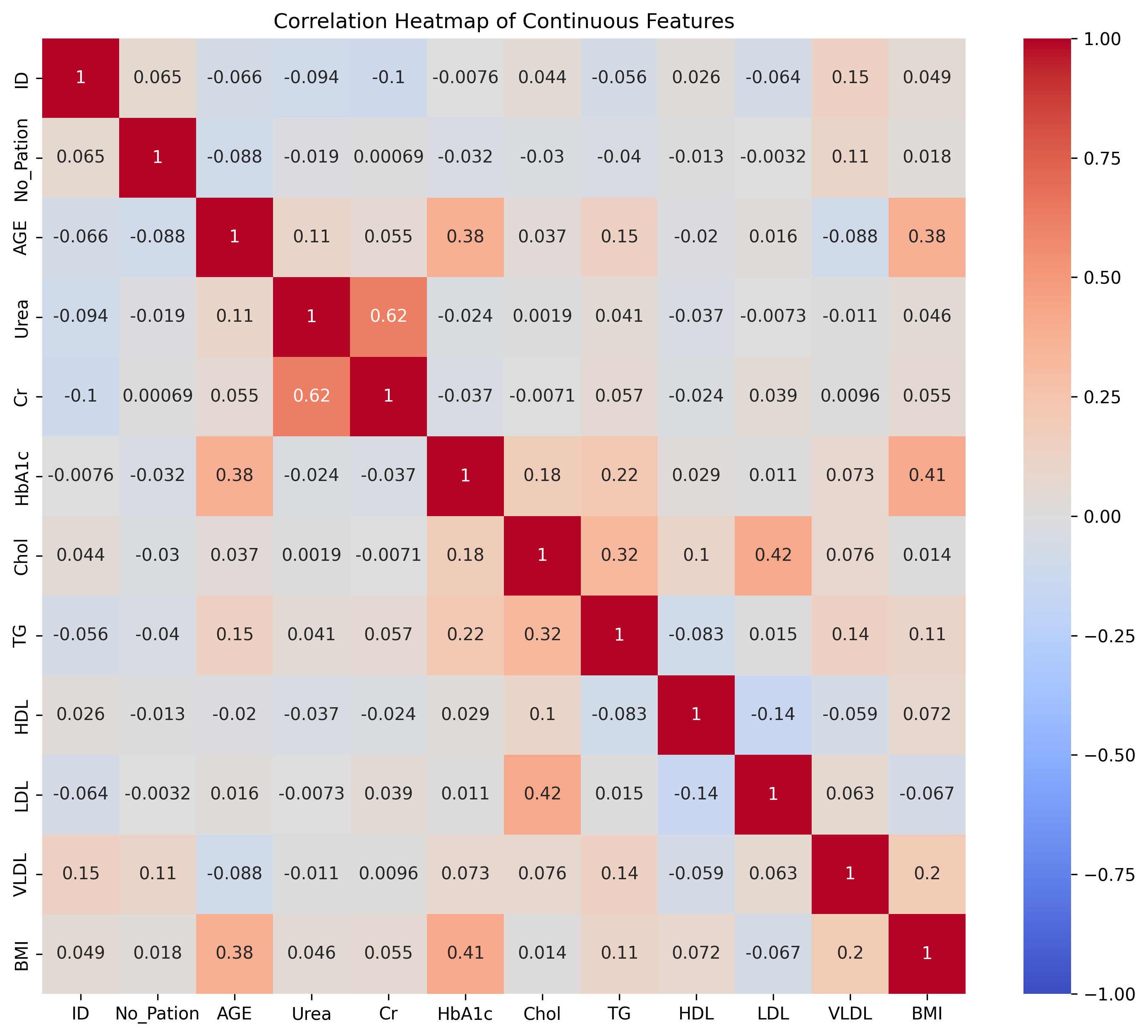
三、连续特征箱线图
# 定义要绘制的特征
features = ['AGE', 'Urea', 'HbA1c', 'Chol', 'TG', 'LDL']"""
创建一个2*3的子图
fig:代表整个2*3的大画布
axes:是一个2*3数组, 通过axes[i][j]访问每个子图
"""
fig, axes = plt.subplots(2, 3, figsize=(12, 8))# 设置分辨率
plt.rcParams['figure.dpi'] = 300# 遍历特征并绘制箱线图 enumerate
for i, feature in enumerate(features):x = i // 3  # 计算当前子图的行索引y = i % 3   # 计算当前子图的列索引# 绘制箱线图 boxplot()axes[x][y].boxplot(dt[feature].dropna())axes[x][y].set_title(f"boxplot of {feature}")axes[x][y].set_ylabel(feature)# 调整布局 tight_layout()
plt.tight_layout()# 显示图形 show()
plt.show()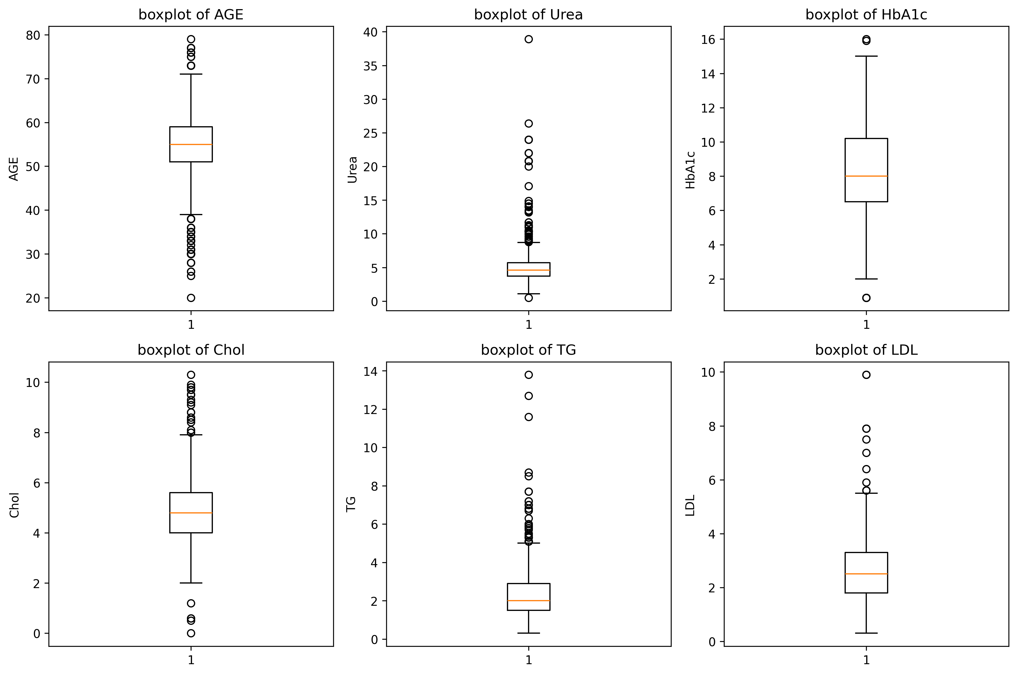
四、模型训练
1、划分数据集
X = dt.drop(['CLASS'], axis=1)   # 特征
y = dt['CLASS']   # 标签
# 8:2划分训练集和测试集
X_train, X_test, y_train, y_test = train_test_split(X, y, test_size=0.2, random_state=42)
2、基准模型
(1)默认随机森林模型
# --- 1.默认参数随机森林模型 ---
print("--- 1.默认参数随机森林模型 ---")
start_time = time.time()
rf_model = RandomForestClassifier(random_state=42)
rf_model.fit(X_train, y_train)
rf_pred = rf_model.predict(X_test)
end_time = time.time()
print(f"随机森林模型训练时间:{end_time - start_time:.4f}, 秒")
print(f"默认随机森林模型准确率:", accuracy_score(y_test, rf_pred))
# !!!该项目是三分类问题,需要修改average参数
print(f"默认随机森林模型f1分数:{f1_score(y_test, rf_pred, average='weighted'):.4f}")
print(f"默认随机森林模型召回率:{recall_score(y_test, rf_pred, average='weighted'):.4f}")
print(f"默认随机森林分类报告:\n", classification_report(y_test, rf_pred))
print(f"默认随机森林混淆矩阵:\n", confusion_matrix(y_test, rf_pred))
print('*' * 55)
输出:
--- 1.默认参数随机森林模型 ---
随机森林模型训练时间:0.1872, 秒
默认随机森林模型准确率: 0.995
默认随机森林模型f1分数:0.9951
默认随机森林模型召回率:0.9950
默认随机森林分类报告:precision    recall  f1-score   support0       0.95      1.00      0.98        211       1.00      1.00      1.00         62       1.00      0.99      1.00       173accuracy                           0.99       200macro avg       0.98      1.00      0.99       200
weighted avg       1.00      0.99      1.00       200默认随机森林混淆矩阵:[[ 21   0   0][  0   6   0][  1   0 172]]
*******************************************************
!!!该项目是三分类问题,需要修改average参数
f1_score参数说明(根据需求选择):
- average='micro' :全局统计TP/FP/FN计算
- average='macro' :各类别平等权重
- average='weighted' :按样本数量加权平均
- average=None :返回每个类别的单独分数
建议使用macro或weighted参数。
(2)默认XGBoost模型
# --- 2.默认参数xgbboost模型 ---
print("--- 2.默认参数xgbboost模型 ---")
start_time = time.time()
xgb_model = xgb.XGBClassifier(random_state=42)
xgb_model.fit(X_train, y_train)
xgb_pred = xgb_model.predict(X_test)
end_time = time.time()
print(f"xgbboost模型训练时间:{end_time - start_time:.4f}, 秒")
print(f"默认xgbboost模型准确率:", accuracy_score(y_test, xgb_pred))
# !!!该项目是三分类问题,需要修改average参数
print(f"默认xgbboost模型f1分数:{f1_score(y_test, xgb_pred, average='weighted'):.4f}")
print(f"默认xgbboost模型召回率:{recall_score(y_test, xgb_pred, average='weighted'):.4f}")
print(f"默认xgbboost分类报告:\n", classification_report(y_test, xgb_pred))
print(f"默认xgbboost混淆矩阵:\n", confusion_matrix(y_test, xgb_pred))
print('*' * 55)
输出:
--- 2.默认参数xgbboost模型 ---
xgbboost模型训练时间:0.2230, 秒
默认xgbboost模型准确率: 0.99
默认xgbboost模型f1分数:0.9900
默认xgbboost模型召回率:0.9900
默认xgbboost分类报告:precision    recall  f1-score   support0       0.95      0.95      0.95        211       1.00      1.00      1.00         62       0.99      0.99      0.99       173accuracy                           0.99       200macro avg       0.98      0.98      0.98       200
weighted avg       0.99      0.99      0.99       200默认xgbboost混淆矩阵:[[ 20   0   1][  0   6   0][  1   0 172]]
*******************************************************
3、处理不平衡数据后的模型
使用smote进行过采样,然后使用随机森林进行分类。
smote = SMOTE(random_state=42)
X_train_smote, y_train_smote = smote.fit_resample(X_train, y_train)
print("SMOTE过采样后训练集的形状:", X_train_smote.shape, y_train_smote.shape)
print("训练集的形状:", X_train.shape, y_train.shape)print("\n--- 3.SMOTE过采样的随机森林模型 ---")
start_time = time.time()
rf_model = RandomForestClassifier(random_state=42)
rf_model.fit(X_train_smote, y_train_smote)
rf_pred = rf_model.predict(X_test)
end_time = time.time()print(f"随机森林模型训练时间:{end_time - start_time:.4f}, 秒")
print(f"默认随机森林分类报告:\n", classification_report(y_test, rf_pred))
print(f"默认随机森林混淆矩阵:\n", confusion_matrix(y_test, rf_pred))
print('*' * 55)
输出:
SMOTE过采样后训练集的形状: (2013, 13) (2013,)
训练集的形状: (800, 13) (800,)--- 3.SMOTE过采样的随机森林模型 ---
随机森林模型训练时间:0.3746, 秒
默认随机森林分类报告:precision    recall  f1-score   support0       0.95      1.00      0.98        211       1.00      1.00      1.00         62       1.00      0.99      1.00       173accuracy                           0.99       200macro avg       0.98      1.00      0.99       200
weighted avg       1.00      0.99      1.00       200默认随机森林混淆矩阵:[[ 21   0   0][  0   6   0][  1   0 172]]
*******************************************************
4、修改权重的随机森林模型
# 关键 定义带权重的模型
rf_model_weighted = RandomForestClassifier(random_state=42,class_weight='balanced'
)
五、可解释性分析 shap图
初始化 SHAP 解释器
# 初始化 SHAP 解释器
explainer = shap.TreeExplainer(rf_model)
shap_values = explainer.shap_values(X_test)
找和测试集形状一样的shap_values输出值
# 找和测试集形状一样的shap_values输出值
print(shap_values[:, :, 0].shape)
print(X_test.shape)
输出:
(200, 13)
(200, 13)
1、SHAP 特征重要性条形图
# --- 1. SHAP 特征重要性条形图 (Summary Plot - Bar) ---
plt.figure(figsize=(10, 6))
shap.summary_plot(shap_values[:, :, 0], X_test, plot_type="bar",show=False) # 只显示第一个类别(0)的条形图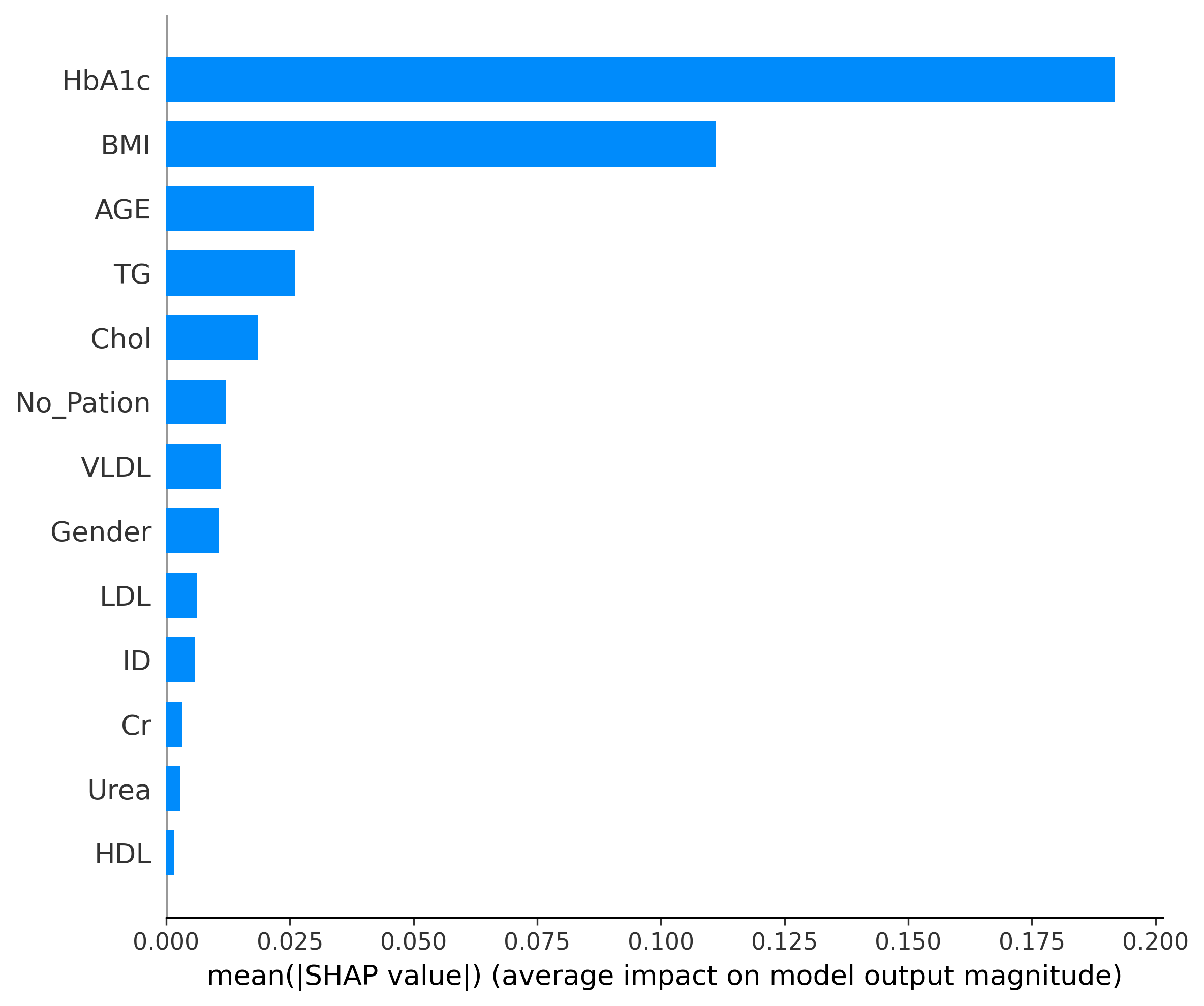
2、特征重要性蜂巢图
shap.summary_plot(shap_values[:, :, 0], X_test, plot_type="violin", show=False)
plt.title("SHAP Feature Importance")
plt.show()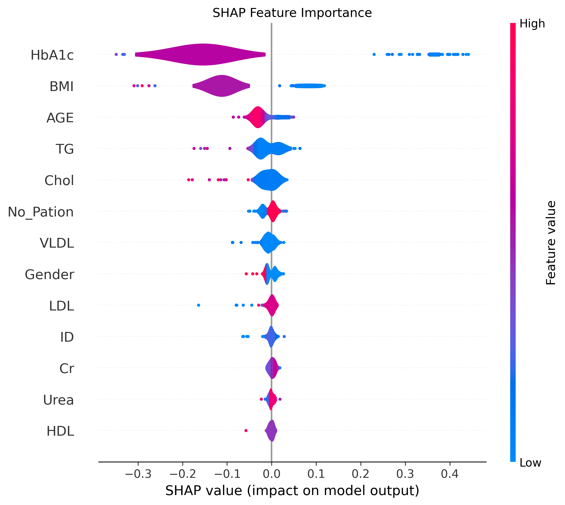
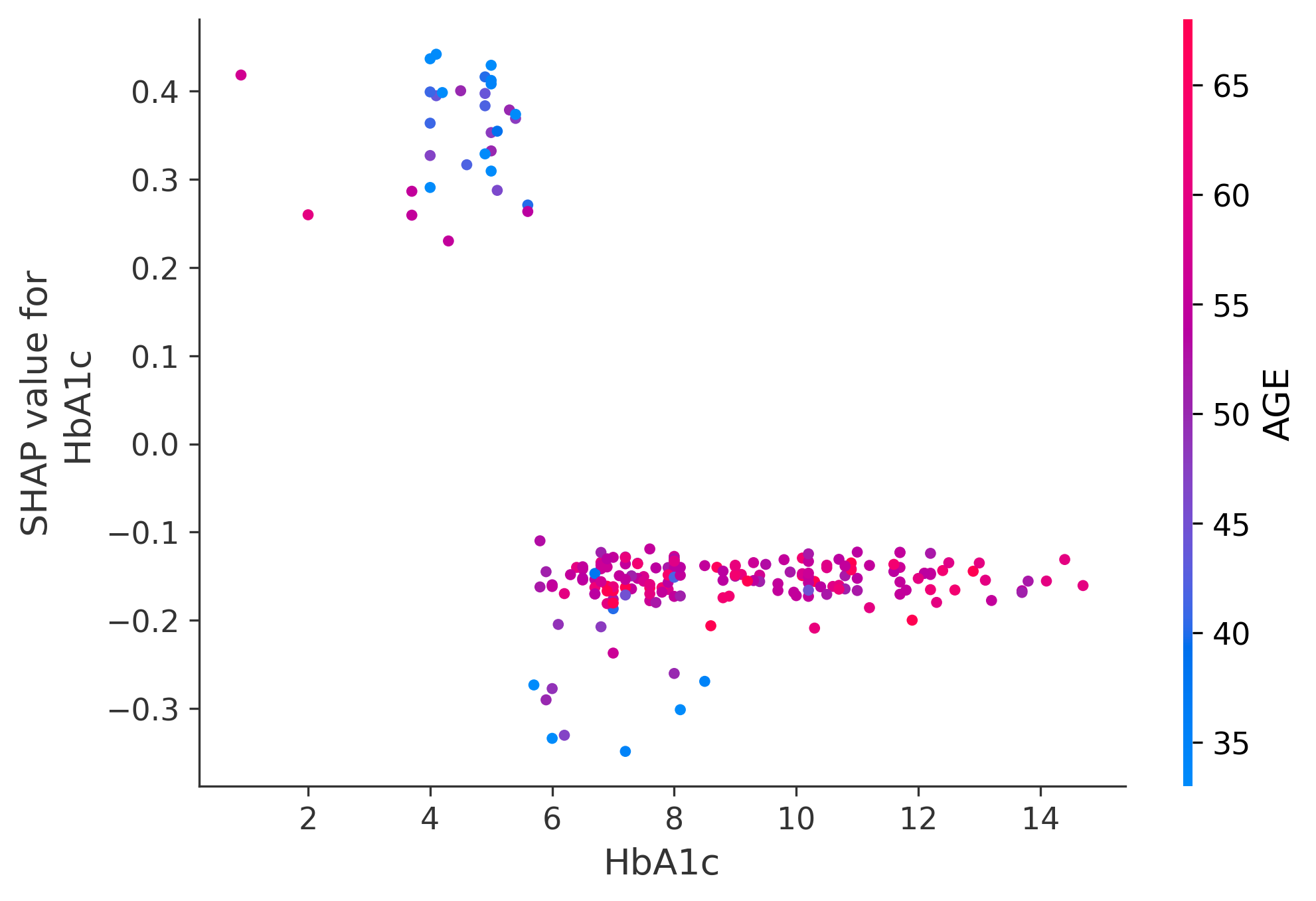
3、SHAP 依赖性图
shap.dependence_plot("BMI", shap_values[:, :, 0], X_test, interaction_index="AGE")
shap.dependence_plot("HbA1c", shap_values[:, :, 0], X_test, interaction_index="AGE")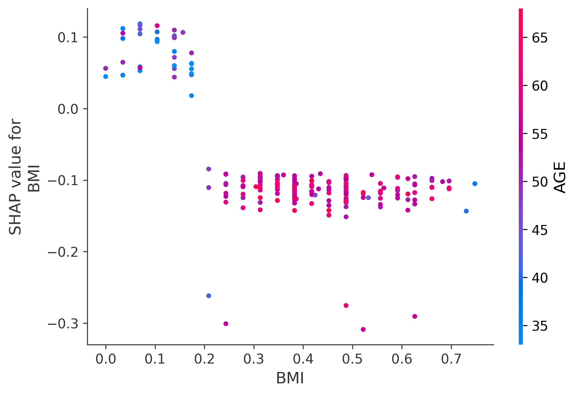
@ 浙大疏锦行