二元Logistic回归
二元Logistic回归
在机器学习领域,二元Logistic回归是一种非常经典的分类模型,广泛用于解决具有两类标签的分类问题。Logistic回归通过逻辑函数(Sigmoid函数)将预测结果映射到概率值,并进行分类。
一、Logistic回归
Logistic回归是一种广泛应用于二分类问题的统计方法,它本质上是一种分类算法。Logistic回归的目标是预测样本属于某一类的概率值。其模型形式为:
p ( y = 1 ∣ X ) = σ ( θ T X ) = 1 1 + e − ( θ T X ) p(y=1|X) = \sigma(\theta^T X) = \frac{1}{1 + e^{-(\theta^T X)}} p(y=1∣X)=σ(θTX)=1+e−(θTX)1
其中, p ( y = 1 ∣ X ) p(y=1|X) p(y=1∣X) 表示给定输入特征 X 时,输出为1的概率, σ ( z ) \sigma(z) σ(z) 为 Sigmoid 函数:
σ ( z ) = 1 1 + e − z \sigma(z) = \frac{1}{1 + e^{-z}} σ(z)=1+e−z1
在二元Logistic回归中, θ \theta θ 是需要学习的模型参数, X X X 是输入特征向量。
二、模型训练
1. 损失函数(Log-Loss)
为了训练Logistic回归模型,我们需要优化一个损失函数,通常采用对数损失函数(Log-Loss),其形式为:
J ( θ ) = − 1 m ∑ i = 1 m [ y ( i ) log ( h θ ( x ( i ) ) ) + ( 1 − y ( i ) ) log ( 1 − h θ ( x ( i ) ) ) ] J(\theta) = -\frac{1}{m} \sum_{i=1}^{m} \left[ y^{(i)} \log(h_{\theta}(x^{(i)})) + (1 - y^{(i)}) \log(1 - h_{\theta}(x^{(i)})) \right] J(θ)=−m1i=1∑m[y(i)log(hθ(x(i)))+(1−y(i))log(1−hθ(x(i)))]
在逻辑回归模型中,假设函数为:
h θ ( x ( i ) ) = σ ( θ T x ( i ) ) h_{\theta}(x^{(i)}) = \sigma(\theta^T x^{(i)}) hθ(x(i))=σ(θTx(i))
其中, h θ ( x ( i ) ) h_{\theta}(x^{(i)}) hθ(x(i)) 是模型的预测结果,m是样本数量, y ( i ) y^{(i)} y(i) 是第i个样本的真实标签。
2. 梯度下降
我们使用梯度下降法来最小化损失函数,更新参数
θ : = θ − α ⋅ ∇ θ J ( θ ) \theta := \theta - \alpha \cdot \nabla_{\theta} J(\theta) θ:=θ−α⋅∇θJ(θ)
其中, α \alpha α 是学习率, ∇ θ J ( θ ) \nabla_{\theta} J(\theta) ∇θJ(θ) 是损失函数的梯度。
三、Python实现
1. 导入必要的库
首先,我们需要导入一些必要的库,例如NumPy用于数学运算,Matplotlib用于绘图等。
import numpy as np
import matplotlib.pyplot as plt
from sklearn.metrics import confusion_matrix
2. 数据加载与预处理
测试样本
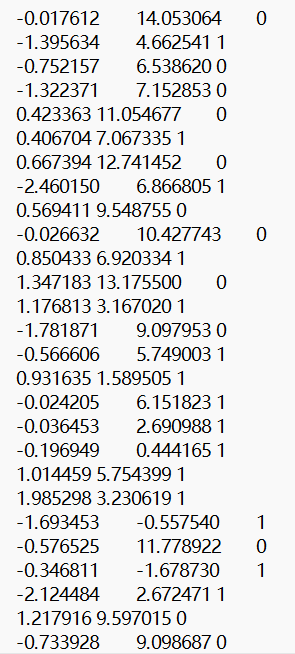
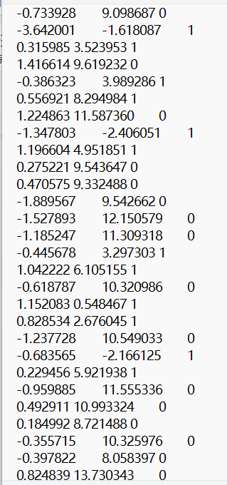
…共一百个样本
数据可视化
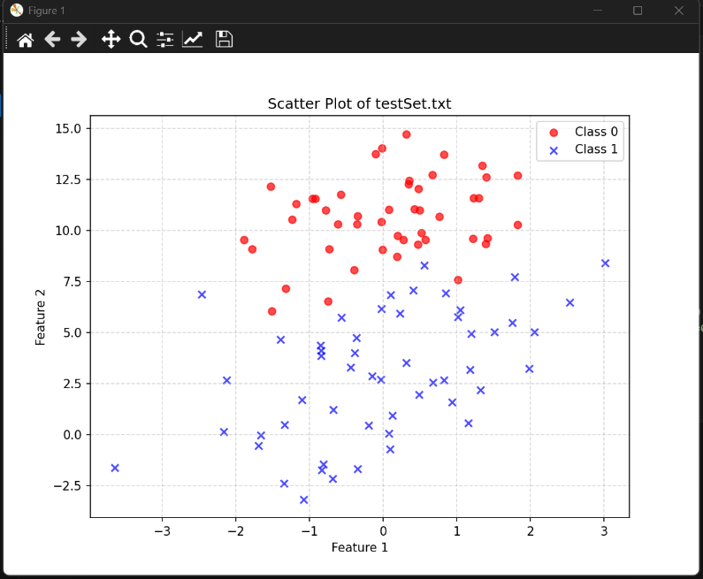
我们假设数据是从一个文本文件中读取,数据的格式为每行包含两个特征和一个标签。
def load_data(file_path):data = np.loadtxt(file_path)X = data[:, 0:2] # 特征y = data[:, 2] # 标签return X, y
3. Sigmoid函数
接下来,定义Sigmoid函数,它将线性模型的输出映射到概率值:
def sigmoid(z):return 1 / (1 + np.exp(-z))
4. 损失函数
然后,我们定义计算对数损失的函数:
def compute_loss(X, y, theta):m = len(y)h = sigmoid(X @ theta) # 预测值loss = -(1/m) * (y @ np.log(h + 1e-15) + (1 - y) @ np.log(1 - h + 1e-15)) # 防止log(0)return loss
5. 梯度下降
我们用梯度下降来训练模型:
def gradient_descent(X, y, theta, alpha, num_iters, tol=1e-5):m = len(y)loss_history = []for i in range(num_iters):h = sigmoid(X @ theta)gradient = (1/m) * X.T @ (h - y) # 计算梯度theta = theta - alpha * gradient # 更新参数loss = compute_loss(X, y, theta)loss_history.append(loss)# 如果损失变化小于tol,停止训练if i > 0 and abs(loss_history[-2] - loss_history[-1]) < tol:print(f"迭代{i}次后损失收敛,停止训练。")breakreturn theta, loss_history
6. 预测函数
我们根据模型的输出概率进行预测,设定阈值为0.5:
def predict(X, theta, threshold=0.5):prob = sigmoid(X @ theta)return (prob >= threshold).astype(int)
7. 主函数
最后,我们将这些步骤组合在一个主函数中,执行数据加载、训练、预测等操作:
if __name__ == "__main__":file_path = "data.txt" # 数据文件路径# 读取数据X, y = load_data(file_path)# 添加偏置项m = X.shape[0]X = np.hstack((np.ones((m, 1)), X))# 参数初始化theta = np.zeros(X.shape[1])# 超参数设置alpha = 0.1num_iters = 1000# 训练模型theta, loss_history = gradient_descent(X, y, theta, alpha, num_iters)print("训练完成,最优参数theta:", theta)# 预测y_pred = predict(X, theta)accuracy = np.mean(y_pred == y)print(f"训练集准确率:{accuracy*100:.2f}%")# 打印混淆矩阵cm = confusion_matrix(y, y_pred)print("混淆矩阵:")print(cm)
四、总结
二元Logistic回归是一种简单且强大的分类算法,广泛应用于许多领域,如医疗诊断、金融欺诈检测等。通过理解其背后的数学原理,并结合Python代码实现,我们可以快速上手并解决实际问题。希望本文能帮助你更好地理解Logistic回归,并能够在实际项目中应用。