当前位置：首页 > news >正文

WRFOUT投影转换——兰伯特转等经纬度

news 来源：原创 2025/5/19 7:17:51

Lambert——WGS84

# -*- coding: utf-8 -*-
import pyproj
import numpy as np
import matplotlib.pyplot as plt
from scipy.interpolate import griddata
import xarray as xr
import geopandas as gpd
import rioxarray  # 用于地理空间操作ds = xr.open_dataset('D:/ZZZZorder_jobs/250508/baseline_d02_205005.nc')  
data = ds['SWDOWN2'][0,:,:]  # 选择你要处理的变量# 输入wrf的网格
x = data.XLONG.data.flatten()  # 经度数据展平为一维数组
y = data.XLAT.data.flatten()   # 纬度数据展平为一维数组
z = data.data.flatten()        # 太阳辐射数据展平为一维数组# 定义Lambert投影和经纬度投影
wrf_proj = pyproj.Proj(proj='lcc', # projection type: Lambert Conformal Coniclat_1=ds.TRUELAT1, lat_2=ds.TRUELAT2, # Cone intersects with the spherelat_0=ds.MOAD_CEN_LAT, lon_0=ds.STAND_LON, # Center pointa=6370000, b=6370000) # This is it! The Earth is a perfect sphere
#等经纬度经纬度投影
wgs_proj = pyproj.Proj(proj='latlong', datum='WGS84')# pyproj.transform() 函数用于将经纬度坐标(ds.CEN_LON, ds.CEN_LAT)从WGS84投影到WRF模型使用的投影坐标系。
e, n = pyproj.transform(wgs_proj, wrf_proj, ds.CEN_LON, ds.CEN_LAT)dx, dy = ds.DX, ds.DY
nx, ny = ds.dims['west_east'], ds.dims['south_north']# 通过计算网格的起始点（左下角）的坐标 x0 和 y0，基于网格的尺寸、分辨率和中心点坐标计算
x0 = -(nx-1) / 2. * dx + e
y0 = -(ny-1) / 2. * dy + n# 用 np.meshgrid() 创建了一个二维网格 (xx, yy)，其中包含了整个模型的网格坐标信息
xx, yy = np.meshgrid(np.arange(nx) * dx + x0, np.arange(ny) * dy + y0)# 使用 pyproj.transform() 将这些网格坐标点从 WRF 模型的投影坐标系转换回经纬度坐标系（PlateCarree投影），结果存储在 our_lons 和 our_lats
our_lons, our_lats = pyproj.transform(wrf_proj, wgs_proj, xx, yy)# 定义插值方法
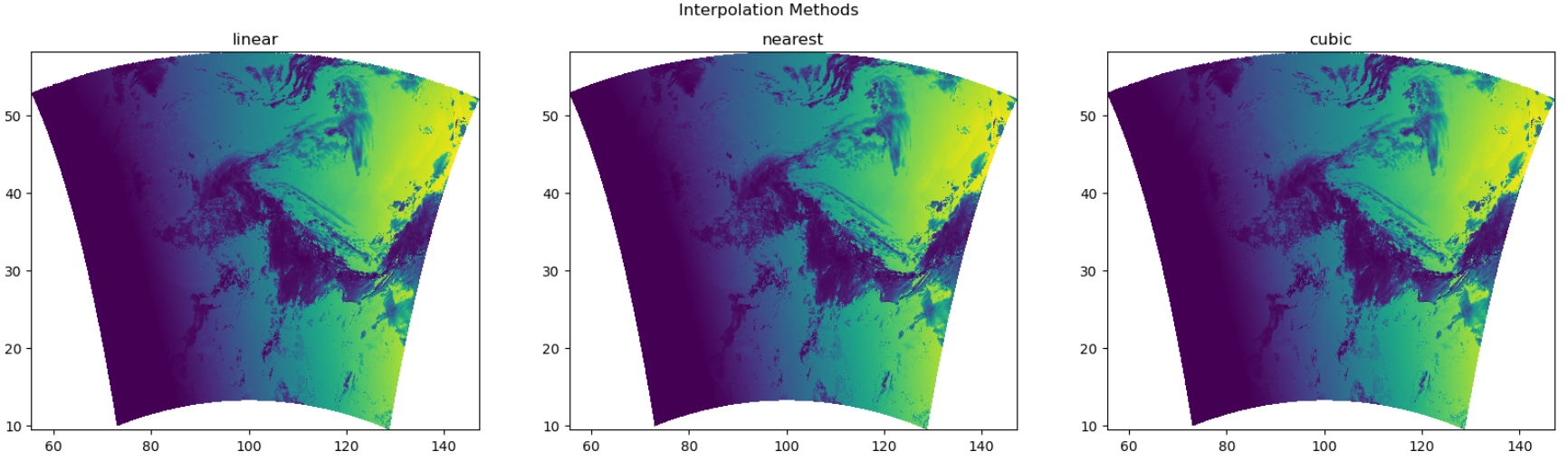
methods = ['linear', 'nearest', 'cubic']# 创建子图
fig, axs = plt.subplots(1, len(methods), figsize=(20, 5))# 进行网格插值并绘制子图
for i, method in enumerate(methods):# 进行网格插值z_target_grid = griddata((x, y), z, (our_lons, our_lats), method=method)# 绘制子图axs[i].pcolormesh(our_lons, our_lats, z_target_grid)axs[i].set_title(method)# 添加颜色条和整体标题
plt.suptitle('Interpolation Methods')
# 显示图形
plt.show()

转换后的下图所示：