当前位置：首页 > news >正文

学习笔记--(7)

news 来源：原创 2025/5/12 5:34:55

粒子物理学习笔记（仅供参考）

import numpy as np
import matplotlib.pyplot as plt
from scipy import constants

# 设置物理常数和绘图风格
plt.style.use('seaborn-poster')
plt.rcParams.update({'font.size': 12})

# QCD β函数系数 (Nf=5)
beta0 = (33 - 2 * 5)/(12*np.pi)
beta1 = (153 - 19 * 5)/(24*np.pi**2)
beta2 = (77139 - 15099 * 5 + 325 * 5**2)/(3456*np.pi**3)
beta3 = (29243 - 6946.3 * 5 + 405.089 * 5**2 + 1.49931 * 5**3)/(256*np.pi**4)

Lambda = 0.220  # Λ_MSbar^(Nf=5) in GeV

# 能量范围 (GeV)
Q = np.logspace(np.log10(1), np.log10(1000), 500)

# 4-loop running coupling (完整表达式)
def alpha_s_4loop(Q, Lambda, Nf=5):
    L = np.log((Q**2)/(Lambda**2))
    a = 1/(beta0*L)
    a -= (beta1/(beta0**3*L**2))*np.log(L)
    a += (1/(beta0**3*L**3)) * ((beta1**2/beta0**2)*(np.log(L)**2 - np.log(L) - 1) + beta2/beta0)
    a += (1/(beta0**4*L**4)) * (
        (beta1**3/beta0**3)*(-np.log(L)**3 + 2.5*np.log(L)**2 + 2*np.log(L) - 0.5) 
        - 3*(beta1*beta2/beta0**2)*np.log(L) 
        + beta3/(2*beta0)
    )
    return a

# 3-loop running coupling (近似)
def alpha_s_3loop(Q, Lambda, Nf=5):
    L = np.log((Q**2)/(Lambda**2))
    a = 1/(beta0*L)
    a -= (beta1/(beta0**3*L**2))*np.log(L)
    a += (1/(beta0**3*L**3)) * ((beta1**2/beta0**2)*(np.log(L)**2 - np.log(L) - 1) + beta2/beta0)
    return a

# 2-loop running coupling
def alpha_s_2loop(Q, Lambda, Nf=5):
    L = np.log((Q**2)/(Lambda**2))
    a = 1/(beta0*L)
    a -= (beta1/(beta0**3*L**2))*np.log(L)
    return a

# 1-loop running coupling
def alpha_s_1loop(Q, Lambda, Nf=5):
    L = np.log((Q**2)/(Lambda**2))
    return 1/(beta0*L)

# 计算不同阶数的αₛ
alpha_1loop = alpha_s_1loop(Q, Lambda)
alpha_2loop = alpha_s_2loop(Q, Lambda)
alpha_3loop = alpha_s_3loop(Q, Lambda)
alpha_4loop = alpha_s_4loop(Q, Lambda)

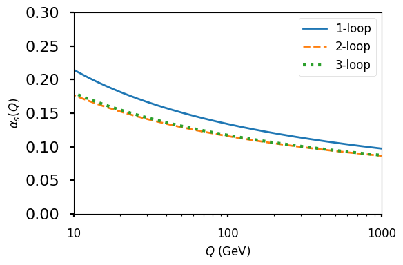
# 创建图形
plt.figure(figsize=(6, 4))

# 绘制曲线
plt.plot(Q, alpha_1loop, '-', linewidth=2, label='1-loop')
plt.plot(Q, alpha_2loop, '--', linewidth=2, label='2-loop')
plt.plot(Q, alpha_3loop, ':', linewidth=3, label='3-loop')
plt.plot(Q, alpha_4loop, '-.', linewidth=2, label='4-loop', color='black')

# 添加标注和装饰
plt.xscale('log')
plt.xlabel(r'$Q$ (GeV)', fontsize=12)
plt.ylabel(r'$\alpha_s(Q)$', fontsize=12)
plt.legend(fontsize=12)
plt.xlim(10, 1000)
plt.xticks([10, 100, 1000], labels=['10', '100', '1000'], fontsize=12)
plt.ylim(0, 0.3)

# 添加注释

# 显示图形
plt.tight_layout()
plt.show()

在这里插入图片描述

import matplotlib.pyplot as plt
import numpy as np
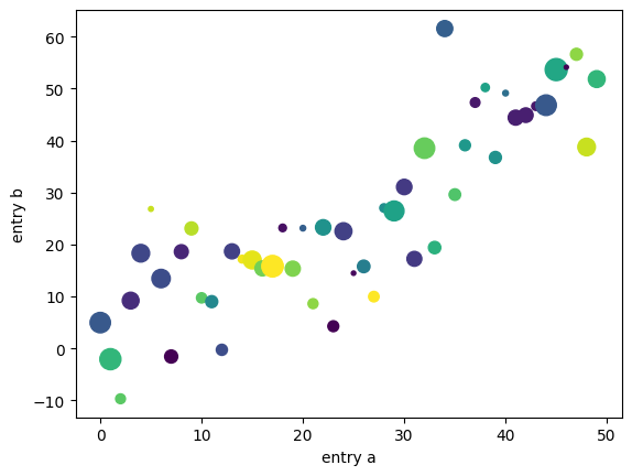
# 使用关键字字符串绘图(data 可指定依赖值为：numpy.recarray 或 pandas.DataFrame）
data = {'a': np.arange(50),  # 1个参数，表示[0,1,2...,50]
        'c': np.random.randint(0, 50, 50),  # 表示产生50个随机数[0,50)
        'd': np.random.randn(50)}  # 返回呈标准正态分布的值（可能正，可能负）
data['b'] = data['a'] + 10 * np.random.randn(50)   
data['d'] = np.abs(data['d']) * 100
plt.scatter('a', 'b', c='c', s='d', data=data)
plt.xlabel('entry a')
plt.ylabel('entry b')
plt.show()