广西金水建设开发有限公司网站参考消息今天新闻

根据论文Factorized Graph Matching学习图分解和图匹配的相关代码，并进行逐行解读

版本1：

优：特征分解、按特征值降序排列特征向量、计算相似度矩阵、匈牙利算法寻找最优匹配

劣：缺少论文中提到的因式分解部分

import numpy as np
from scipy.optimize import linear_sum_assignment# 用于接收两个邻接矩阵，A/B表示待匹配的图
def factorized_graph_matching(A, B):# 对邻接矩阵进行特征分解 np.linalg.eigh()函数专门用于对称矩阵# 结果是得到矩阵的特征值eigvals和对应的特征向量eigvecseigvals_A, eigvecs_A = np.linalg.eigh(A)eigvals_B, eigvecs_B = np.linalg.eigh(B)# 按特征值降序排列特征向量（处理符号问题）# 特征值降序排列返回索引idx_A = np.argsort(eigvals_A)[::-1]# 通过索引对特征向量重排eigvecs_A = eigvecs_A[:, idx_A]# 图解过程 标准化特征向量符号eigvecs_A = np.sign(eigvecs_A[np.argmax(np.abs(eigvecs_A), axis=0), range(eigvecs_A.shape[1])]) * eigvecs_Aidx_B = np.argsort(eigvals_B)[::-1]eigvecs_B = eigvecs_B[:, idx_B]eigvecs_B = np.sign(eigvecs_B[np.argmax(np.abs(eigvecs_B), axis=0), range(eigvecs_B.shape[1])]) * eigvecs_B# 计算特征向量间的相似度矩阵（余弦相似度）similarity = np.abs(eigvecs_A.T @ eigvecs_B)# 使用匈牙利算法寻找最优匹配（负号，默认最小代价但希望最大相似度）row_ind, col_ind = linear_sum_assignment(-similarity)# 构建匹配结果matching = np.zeros(A.shape[0], dtype=int)matching[row_ind] = col_indreturn matching# 示例用法
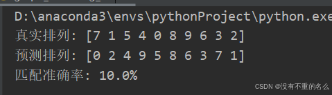
if __name__ == "__main__":np.random.seed(0)n = 5  # 节点数量# 生成原始图A和其排列版本B（添加噪声）A = np.random.rand(n, n)A = (A + A.T) / 2  # 对称化true_perm = np.random.permutation(n)B = A[true_perm][:, true_perm]B += np.random.normal(scale=0.05, size=(n, n))  # 添加噪声# 进行图匹配predicted_perm = factorized_graph_matching(A, B)# 显示结果print("真实排列:", true_perm)print("预测排列:", predicted_perm)accuracy = np.mean(predicted_perm == true_perm)print(f"匹配准确率: {accuracy * 100:.1f}%")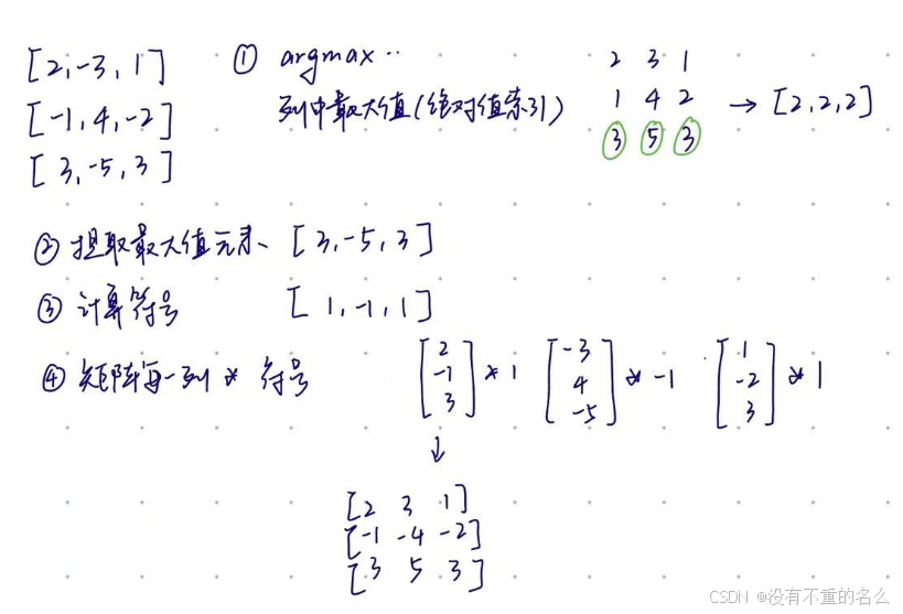

 ①随机生成矩阵A

②对称化，便于使用np.linalg.eigh()函数，专门用于对称矩阵

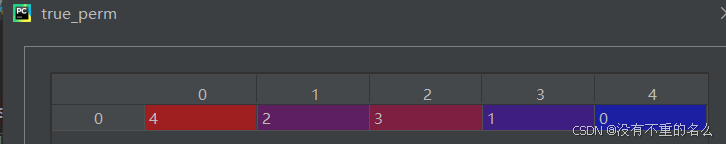
③生成一个随机重排列，用于生成B，并添加扰动噪声

 ④跳入函数进行匹配

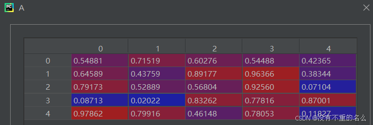
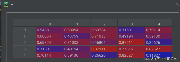
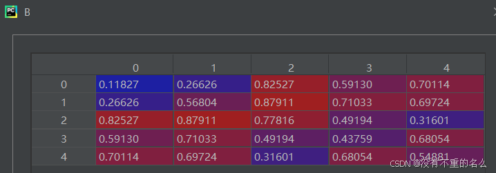
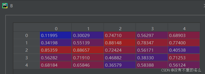
输入：

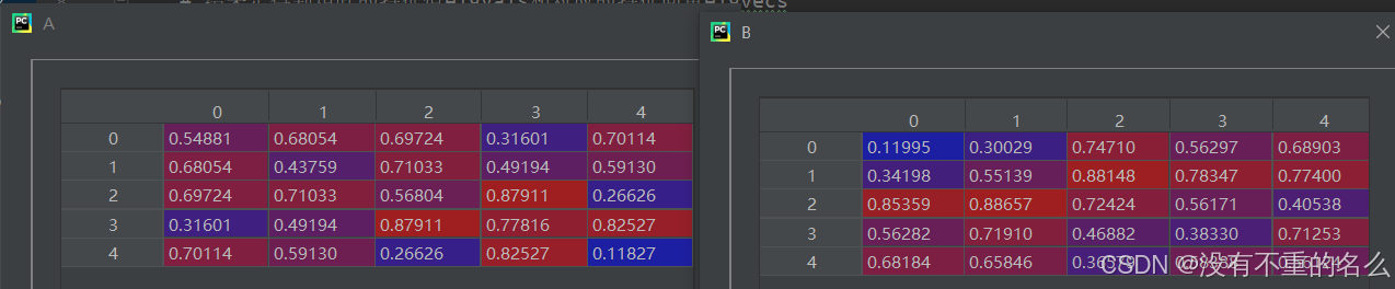
 提取AB的特征值和特征向量：

特征值降序返回索引：

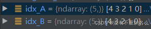
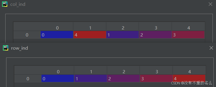
通过索引对特征值和特征向量重排：

 计算特征向量之间的相似度：

 匈牙利算法寻找最优匹配：

 构建0矩阵，填入匹配结果

版本2：

优：适用于小规模图的匹配任务，手动分块

劣：通过Euclidean距离来计算每个节点之间的相似度，使用了节点的属性值进行匹配

import numpy as np
import networkx as nx
from scipy.optimize import linear_sum_assignmentdef compute_cost_matrix(graph1, graph2):# 获取节点数量num_nodes1 = len(graph1.nodes)num_nodes2 = len(graph2.nodes)# 初始化全为0的代价矩阵cost_matrix = np.zeros((num_nodes1, num_nodes2))# 遍历两个图的每个节点for i, node1 in enumerate(graph1.nodes):for j, node2 in enumerate(graph2.nodes):# 从图中获取节点特征值，若没有特征值设为0value1 = graph1.nodes[node1].get('value', np.array([0]))value2 = graph2.nodes[node2].get('value', np.array([0]))# 计算两个节点特征值之间的欧几里得距离，并将其作为匹配代价存入代价矩阵cost_matrix[i, j] = np.linalg.norm(value1 - value2)return cost_matrixdef factorized_graph_matching(graph1, graph2):# Step 1: 计算两个图之间的代价矩阵cost_matrix = compute_cost_matrix(graph1, graph2)# Step 2: 使用匈牙利算法求解代价矩阵的最优匹配row_ind, col_ind = linear_sum_assignment(cost_matrix)# Step 3: 将匹配结果组合成一个列表matching = list(zip(row_ind, col_ind))return matchingdef create_sample_graph():graph1 = nx.Graph()# 创建一个包含三个节点（编号为0，1，2）的图1graph1.add_nodes_from([0, 1, 2])# 为每个节点添加一个名为value的属性graph1.nodes[0]['value'] = np.array([1, 2])graph1.nodes[1]['value'] = np.array([2, 3])graph1.nodes[2]['value'] = np.array([3, 4])graph2 = nx.Graph()graph2.add_nodes_from([0, 1, 2])graph2.nodes[0]['value'] = np.array([1, 1])graph2.nodes[1]['value'] = np.array([2, 2])graph2.nodes[2]['value'] = np.array([3, 3])return graph1, graph2if __name__ == "__main__":graph1, graph2 = create_sample_graph()matching = factorized_graph_matching(graph1, graph2)print("Optimal Node Matching:")for node1, node2 in matching:print(f"Graph1 Node {node1} is matched with Graph2 Node {node2}")

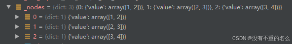
①创建两张图，并为节点赋予属性值

graph1：

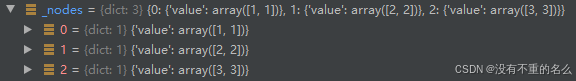
graph2： 

②调用图匹配函数，匹配graph1和graph2

step1：计算两个图之间的代价矩阵

1.获取节点数量并初始化代价矩阵

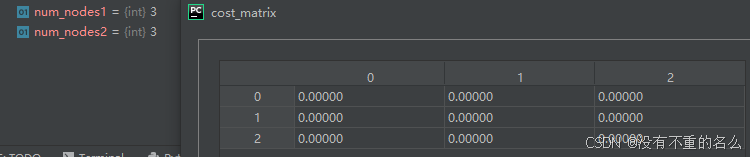
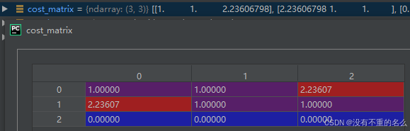
2. 遍历两个图的每个节点并获取节点特征值，若没有特征值则设为0；计算代价矩阵

代价越小，对应的匹配越优 

 step2：使用匈牙利算法求解代价矩阵的最优匹配

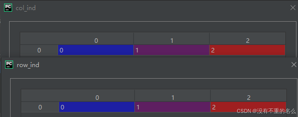
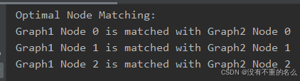
step3： 将匹配结果组合成一个列表

得到匹配结果

版本3：

结合上述两种

import numpy as np
import networkx as nx
from scipy.optimize import linear_sum_assignment# 将输入图转换为邻接矩阵
def compute_adjacency_matrix(graph):return nx.to_numpy_array(graph)def factorized_graph_matching(graph1, graph2, k=5):# Step 1: 计算邻接矩阵A1 = compute_adjacency_matrix(graph1)A2 = compute_adjacency_matrix(graph2)# Step 2: 计算特征值和特征向量eigvals_A1, eigvecs_A1 = np.linalg.eigh(A1)eigvals_A2, eigvecs_A2 = np.linalg.eigh(A2)# Step 3: 按特征值降序排列特征向量idx_A1 = np.argsort(eigvals_A1)[::-1]eigvecs_A1 = eigvecs_A1[:, idx_A1]idx_A2 = np.argsort(eigvals_A2)[::-1]eigvecs_A2 = eigvecs_A2[:, idx_A2]# Step 4: 选择前k个特征向量（更具有代表性）eigvecs_A1 = eigvecs_A1[:, :k]eigvecs_A2 = eigvecs_A2[:, :k]# Step 5: 计算特征向量之间的相似度矩阵similarity_matrix = np.abs(np.dot(eigvecs_A1.T, eigvecs_A2))# Step 6: 使用匈牙利算法找到最优匹配row_ind, col_ind = linear_sum_assignment(-similarity_matrix)# Step 7: 返回匹配结果matching = list(zip(row_ind, col_ind))return matchingdef create_sample_graph():graph1 = nx.Graph()graph1.add_nodes_from([0, 1, 2, 3])graph1.add_edges_from([(0, 1), (1, 2), (2, 3)])graph2 = nx.Graph()graph2.add_nodes_from([0, 1, 2, 3])graph2.add_edges_from([(0, 2), (1, 3), (2, 3)])return graph1, graph2# Test the factorized graph matching
if __name__ == "__main__":graph1, graph2 = create_sample_graph()matching = factorized_graph_matching(graph1, graph2, k=2)print("Optimal Node Matching:")for node1, node2 in matching:print(f"Graph1 Node {node1} is matched with Graph2 Node {node2}")

版本4：

使用SVD，和论文基本一致的因式分解

SVD分解函数：

import numpy as npdef factorize_cost_matrix(K, rank=2):# K：需要分解的矩阵 U：左因子矩阵 sigma：奇异值矩阵（对角矩阵） V：右因子矩阵# Step 1：对矩阵K进行奇异值分解U, sigma, Vt = np.linalg.svd(K, full_matrices=False)# Step 2：保留前rank个奇异值和对应的奇异向量# 从U中提取前rank列，表示保留的左奇异向量。U = U[:, :rank]  # 从奇异值数组中提取前rank个奇异值，并将它们转换为对角矩阵Σ。sigma = np.diag(sigma[:rank])  # 从VT的转置中提取前 rank 列，表示保留的右奇异向量V = Vt.T[:, :rank]  return U, sigma, V# Example usage:
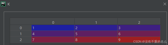
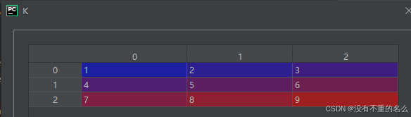
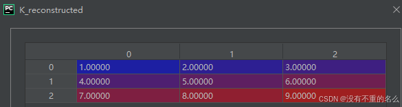
if __name__ == "__main__":# Example cost matrix K (could be a similarity or distance matrix)K = np.array([[1, 2, 3], [4, 5, 6], [7, 8, 9]])# Factorize the cost matrix into U and VU, sigma, V = factorize_cost_matrix(K, rank=2)# Reconstruct the matrix K from U, sigma, and VK_reconstructed = U @ sigma @ V.Tprint("Original Matrix K:")print(K)print("\nReconstructed Matrix K:")print(K_reconstructed)

①传入分解的矩阵K

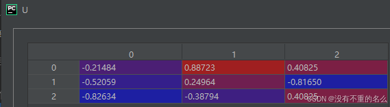
 ②对矩阵K进行奇异值分解

 ③保留前rank个奇异值和对应的奇异向量

低秩近似：通过保留矩阵的主要成分来近似原始矩阵，同时减少计算复杂度和数据维度

SVD分解可以表示为：

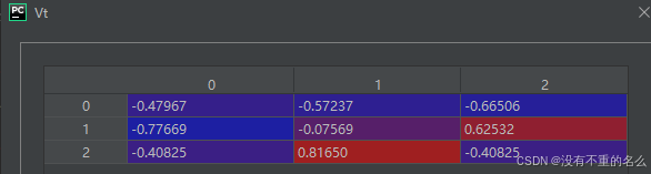
，：正交矩阵

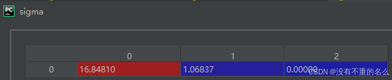
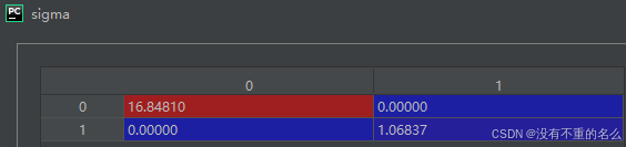
：对角矩阵，对角线上的元素是奇异值，按从大到小的顺序排列

奇异值的大小反映了矩阵中每个成分的重要性。较大的奇异值对应于矩阵的主要结构信息，而较小的奇异值通常可以被视为噪声或次要信息

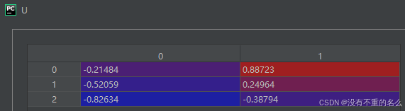
左奇异向量：

 对角矩阵Σ：

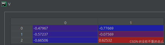
 右奇异向量：

 ④重塑K

结合SVD后的图匹配：

import numpy as np
import networkx as nx
from scipy.optimize import linear_sum_assignment# 计算节点间的相似度矩阵
def compute_similarity_matrix(graph1, graph2):"""计算两个图之间的节点相似度矩阵。这里使用欧几里得距离来计算节点之间的相似度。"""num_nodes1 = len(graph1.nodes)num_nodes2 = len(graph2.nodes)# 初始化相似度矩阵similarity_matrix = np.zeros((num_nodes1, num_nodes2))# 计算节点间的相似度（以欧几里得距离为例）for i, node1 in enumerate(graph1.nodes):for j, node2 in enumerate(graph2.nodes):# 假设每个节点有一个'value'属性，我们用该属性进行相似度计算value1 = graph1.nodes[node1].get('value', np.array([0]))value2 = graph2.nodes[node2].get('value', np.array([0]))# 使用欧几里得距离作为相似度（可以替换为其他相似度度量方法）similarity_matrix[i, j] = np.linalg.norm(value1 - value2)return similarity_matrix# 使用SVD进行因式分解
def factorize_cost_matrix(K, rank=2):"""使用SVD对代价矩阵K进行因式分解。"""# 对K矩阵进行SVD分解U, sigma, Vt = np.linalg.svd(K, full_matrices=False)# 保留前rank个奇异值U = U[:, :rank]sigma = np.diag(sigma[:rank])V = Vt.T[:, :rank]return U, sigma, V# 图匹配函数
def factorized_graph_matching(graph1, graph2, rank=2):"""使用因式分解方法进行图匹配。"""# 计算节点相似度矩阵（代价矩阵）similarity_matrix = compute_similarity_matrix(graph1, graph2)# 使用SVD进行因式分解U, sigma, V = factorize_cost_matrix(similarity_matrix, rank)# 重构代价矩阵reconstructed_matrix = U @ sigma @ V.T# 使用匈牙利算法进行最优匹配row_ind, col_ind = linear_sum_assignment(reconstructed_matrix)# 输出匹配结果matching = list(zip(row_ind, col_ind))return matching# 创建样本图
def create_sample_graph():"""创建测试用的样本图。图中每个节点都有一个'value'属性，用于计算相似度。"""graph1 = nx.Graph()graph1.add_nodes_from([0, 1, 2])graph1.nodes[0]['value'] = np.array([1, 2])graph1.nodes[1]['value'] = np.array([2, 3])graph1.nodes[2]['value'] = np.array([3, 4])graph2 = nx.Graph()graph2.add_nodes_from([0, 1, 2])graph2.nodes[0]['value'] = np.array([1, 1])graph2.nodes[1]['value'] = np.array([2, 2])graph2.nodes[2]['value'] = np.array([3, 3])return graph1, graph2# 测试图匹配
if __name__ == "__main__":# 创建样本图graph1, graph2 = create_sample_graph()# 进行图匹配matching = factorized_graph_matching(graph1, graph2)# 输出匹配结果print("Optimal Node Matching:")for node1, node2 in matching:print(f"Graph1 Node {node1} is matched with Graph2 Node {node2}")