第18周:YOLOv5-C3模块实现
目录
前言
一、 前期准备
1. 设置GPU
2. 导入数据
3. 划分数据集
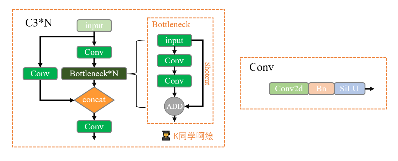
二、搭建包含C3模块的模型
1. 搭建模型
2. 查看模型详情
三、 训练模型
1. 编写训练函数
2. 编写测试函数
3. 正式训练
四、 结果可视化
1. Loss与Accuracy图
2. 模型评估
五、总结
前言
- 🍨 本文为🔗365天深度学习训练营中的学习记录博客
- 🍖 原作者:K同学啊
一、 前期准备
1. 设置GPU
import torch
import torch.nn as nn
import torchvision.transforms as transforms
import torchvision
from torchvision import transforms, datasets
import os,PIL,pathlib,warnings

warnings.filterwarnings("ignore")             #忽略警告信息

device = torch.device("cuda" if torch.cuda.is_available() else "cpu")
device
2. 导入数据
import os,PIL,random,pathlib

data_dir = './8-data/'
data_dir = pathlib.Path(data_dir)

data_paths  = list(data_dir.glob('*'))
classeNames = [str(path).split("\\")[1] for path in data_paths]
classeNames
['cloudy', 'rain', 'shine', 'sunrise']
# 关于transforms.Compose的更多介绍可以参考:https://blog.csdn.net/qq_38251616/article/details/124878863
train_transforms = transforms.Compose([
    transforms.Resize([224, 224]),  # 将输入图片resize成统一尺寸
    # transforms.RandomHorizontalFlip(), # 随机水平翻转
    transforms.ToTensor(),          # 将PIL Image或numpy.ndarray转换为tensor,并归一化到[0,1]之间
    transforms.Normalize(           # 标准化处理-->转换为标准正太分布(高斯分布),使模型更容易收敛
        mean=[0.485, 0.456, 0.406],
        std=[0.229, 0.224, 0.225])  # 其中 mean=[0.485,0.456,0.406]与std=[0.229,0.224,0.225] 从数据集中随机抽样计算得到的。
])

test_transform = transforms.Compose([
    transforms.Resize([224, 224]),  # 将输入图片resize成统一尺寸
    transforms.ToTensor(),          # 将PIL Image或numpy.ndarray转换为tensor,并归一化到[0,1]之间
    transforms.Normalize(           # 标准化处理-->转换为标准正太分布(高斯分布),使模型更容易收敛
        mean=[0.485, 0.456, 0.406],
        std=[0.229, 0.224, 0.225])  # 其中 mean=[0.485,0.456,0.406]与std=[0.229,0.224,0.225] 从数据集中随机抽样计算得到的。
])

total_data = datasets.ImageFolder("./8-data/",transform=train_transforms)
total_data
Dataset ImageFolder
Number of datapoints: 1125
Root location: ./8-data/
StandardTransform
Transform: Compose(
Resize(size=[224, 224], interpolation=bilinear, max_size=None, antialias=None)
ToTensor()
Normalize(mean=[0.485, 0.456, 0.406], std=[0.229, 0.224, 0.225])
)
total_data.class_to_idx{'cloudy': 0, 'rain': 1, 'shine': 2, 'sunrise': 3}
3. 划分数据集
train_size = int(0.8 * len(total_data))
test_size  = len(total_data) - train_size
train_dataset, test_dataset = torch.utils.data.random_split(total_data, [train_size, test_size])
train_dataset, test_dataset
(<torch.utils.data.dataset.Subset at 0x19600429450>,
<torch.utils.data.dataset.Subset at 0x196004297e0>)
batch_size = 4

train_dl = torch.utils.data.DataLoader(train_dataset,
                                           batch_size=batch_size,
                                           shuffle=True,
                                           num_workers=1)
test_dl = torch.utils.data.DataLoader(test_dataset,
                                          batch_size=batch_size,
                                          shuffle=True,
                                          num_workers=1)
for X, y in test_dl:
print("Shape of X [N, C, H, W]: ", X.shape)
print("Shape of y: ", y.shape, y.dtype)
breakShape of X [N, C, H, W]: torch.Size([4, 3, 224, 224])
Shape of y: torch.Size([4]) torch.int64
二、搭建包含C3模块的模型
1. 搭建模型
import torch.nn.functional as F

def autopad(k, p=None):  # kernel, padding
    # Pad to 'same'
    if p is None:
        p = k // 2 if isinstance(k, int) else [x // 2 for x in k]  # auto-pad
    return p

class Conv(nn.Module):
    # Standard convolution
    def __init__(self, c1, c2, k=1, s=1, p=None, g=1, act=True):  # ch_in, ch_out, kernel, stride, padding, groups
        super().__init__()
        self.conv = nn.Conv2d(c1, c2, k, s, autopad(k, p), groups=g, bias=False)
        self.bn = nn.BatchNorm2d(c2)
        self.act = nn.SiLU() if act is True else (act if isinstance(act, nn.Module) else nn.Identity())

    def forward(self, x):
        return self.act(self.bn(self.conv(x)))

class Bottleneck(nn.Module):
    # Standard bottleneck
    def __init__(self, c1, c2, shortcut=True, g=1, e=0.5):  # ch_in, ch_out, shortcut, groups, expansion
        super().__init__()
        c_ = int(c2 * e)  # hidden channels
        self.cv1 = Conv(c1, c_, 1, 1)
        self.cv2 = Conv(c_, c2, 3, 1, g=g)
        self.add = shortcut and c1 == c2

    def forward(self, x):
        return x + self.cv2(self.cv1(x)) if self.add else self.cv2(self.cv1(x))

class C3(nn.Module):
    # CSP Bottleneck with 3 convolutions
    def __init__(self, c1, c2, n=1, shortcut=True, g=1, e=0.5):  # ch_in, ch_out, number, shortcut, groups, expansion
        super().__init__()
        c_ = int(c2 * e)  # hidden channels
        self.cv1 = Conv(c1, c_, 1, 1)
        self.cv2 = Conv(c1, c_, 1, 1)
        self.cv3 = Conv(2 * c_, c2, 1)  # act=FReLU(c2)
        self.m = nn.Sequential(*(Bottleneck(c_, c_, shortcut, g, e=1.0) for _ in range(n)))

    def forward(self, x):
        return self.cv3(torch.cat((self.m(self.cv1(x)), self.cv2(x)), dim=1))

class model_K(nn.Module):
    def __init__(self):
        super(model_K, self).__init__()

        # 卷积模块
        self.Conv = Conv(3, 32, 3, 2)

        # C3模块1
        self.C3_1 = C3(32, 64, 3, 2)

        # 全连接网络层,用于分类
        self.classifier = nn.Sequential(
            nn.Linear(in_features=802816, out_features=100),
            nn.ReLU(),
            nn.Linear(in_features=100, out_features=4)
        )

    def forward(self, x):
        x = self.Conv(x)
        x = self.C3_1(x)
        x = torch.flatten(x, start_dim=1)
        x = self.classifier(x)

        return x

device = "cuda" if torch.cuda.is_available() else "cpu"
print("Using {} device".format(device))

model = model_K().to(device)
model
Using cuda device
model_K(
(Conv): Conv(
(conv): Conv2d(3, 32, kernel_size=(3, 3), stride=(2, 2), padding=(1, 1), bias=False)
(bn): BatchNorm2d(32, eps=1e-05, momentum=0.1, affine=True, track_running_stats=True)
(act): SiLU()
)
(C3_1): C3(
(cv1): Conv(
(conv): Conv2d(32, 32, kernel_size=(1, 1), stride=(1, 1), bias=False)
(bn): BatchNorm2d(32, eps=1e-05, momentum=0.1, affine=True, track_running_stats=True)
(act): SiLU()
)
(cv2): Conv(
(conv): Conv2d(32, 32, kernel_size=(1, 1), stride=(1, 1), bias=False)
(bn): BatchNorm2d(32, eps=1e-05, momentum=0.1, affine=True, track_running_stats=True)
(act): SiLU()
)
(cv3): Conv(
(conv): Conv2d(64, 64, kernel_size=(1, 1), stride=(1, 1), bias=False)
(bn): BatchNorm2d(64, eps=1e-05, momentum=0.1, affine=True, track_running_stats=True)
(act): SiLU()
)
(m): Sequential(
(0): Bottleneck(
(cv1): Conv(
(conv): Conv2d(32, 32, kernel_size=(1, 1), stride=(1, 1), bias=False)
(bn): BatchNorm2d(32, eps=1e-05, momentum=0.1, affine=True, track_running_stats=True)
(act): SiLU()
)
(cv2): Conv(
(conv): Conv2d(32, 32, kernel_size=(3, 3), stride=(1, 1), padding=(1, 1), bias=False)
(bn): BatchNorm2d(32, eps=1e-05, momentum=0.1, affine=True, track_running_stats=True)
(act): SiLU()
)
)
(1): Bottleneck(
(cv1): Conv(
(conv): Conv2d(32, 32, kernel_size=(1, 1), stride=(1, 1), bias=False)
(bn): BatchNorm2d(32, eps=1e-05, momentum=0.1, affine=True, track_running_stats=True)
(act): SiLU()
)
(cv2): Conv(
(conv): Conv2d(32, 32, kernel_size=(3, 3), stride=(1, 1), padding=(1, 1), bias=False)
(bn): BatchNorm2d(32, eps=1e-05, momentum=0.1, affine=True, track_running_stats=True)
(act): SiLU()
)
)
(2): Bottleneck(
(cv1): Conv(
(conv): Conv2d(32, 32, kernel_size=(1, 1), stride=(1, 1), bias=False)
(bn): BatchNorm2d(32, eps=1e-05, momentum=0.1, affine=True, track_running_stats=True)
(act): SiLU()
)
(cv2): Conv(
(conv): Conv2d(32, 32, kernel_size=(3, 3), stride=(1, 1), padding=(1, 1), bias=False)
(bn): BatchNorm2d(32, eps=1e-05, momentum=0.1, affine=True, track_running_stats=True)
(act): SiLU()
)
)
)
)
(classifier): Sequential(
(0): Linear(in_features=802816, out_features=100, bias=True)
(1): ReLU()
(2): Linear(in_features=100, out_features=4, bias=True)
)
)
2. 查看模型详情
# 统计模型参数量以及其他指标
import torchsummary as summary
summary.summary(model, (3, 224, 224))
----------------------------------------------------------------
Layer (type) Output Shape Param #
================================================================
Conv2d-1 [-1, 32, 112, 112] 864
BatchNorm2d-2 [-1, 32, 112, 112] 64
SiLU-3 [-1, 32, 112, 112] 0
Conv-4 [-1, 32, 112, 112] 0
Conv2d-5 [-1, 32, 112, 112] 1,024
BatchNorm2d-6 [-1, 32, 112, 112] 64
SiLU-7 [-1, 32, 112, 112] 0
Conv-8 [-1, 32, 112, 112] 0
Conv2d-9 [-1, 32, 112, 112] 1,024
BatchNorm2d-10 [-1, 32, 112, 112] 64
SiLU-11 [-1, 32, 112, 112] 0
Conv-12 [-1, 32, 112, 112] 0
Conv2d-13 [-1, 32, 112, 112] 9,216
BatchNorm2d-14 [-1, 32, 112, 112] 64
SiLU-15 [-1, 32, 112, 112] 0
Conv-16 [-1, 32, 112, 112] 0
Bottleneck-17 [-1, 32, 112, 112] 0
Conv2d-18 [-1, 32, 112, 112] 1,024
BatchNorm2d-19 [-1, 32, 112, 112] 64
SiLU-20 [-1, 32, 112, 112] 0
Conv-21 [-1, 32, 112, 112] 0
Conv2d-22 [-1, 32, 112, 112] 9,216
BatchNorm2d-23 [-1, 32, 112, 112] 64
SiLU-24 [-1, 32, 112, 112] 0
Conv-25 [-1, 32, 112, 112] 0
Bottleneck-26 [-1, 32, 112, 112] 0
Conv2d-27 [-1, 32, 112, 112] 1,024
BatchNorm2d-28 [-1, 32, 112, 112] 64
SiLU-29 [-1, 32, 112, 112] 0
Conv-30 [-1, 32, 112, 112] 0
Conv2d-31 [-1, 32, 112, 112] 9,216
BatchNorm2d-32 [-1, 32, 112, 112] 64
SiLU-33 [-1, 32, 112, 112] 0
Conv-34 [-1, 32, 112, 112] 0
Bottleneck-35 [-1, 32, 112, 112] 0
Conv2d-36 [-1, 32, 112, 112] 1,024
BatchNorm2d-37 [-1, 32, 112, 112] 64
SiLU-38 [-1, 32, 112, 112] 0
Conv-39 [-1, 32, 112, 112] 0
Conv2d-40 [-1, 64, 112, 112] 4,096
BatchNorm2d-41 [-1, 64, 112, 112] 128
SiLU-42 [-1, 64, 112, 112] 0
Conv-43 [-1, 64, 112, 112] 0
C3-44 [-1, 64, 112, 112] 0
Linear-45 [-1, 100] 80,281,700
ReLU-46 [-1, 100] 0
Linear-47 [-1, 4] 404
================================================================
Total params: 80,320,536
Trainable params: 80,320,536
Non-trainable params: 0
----------------------------------------------------------------
Input size (MB): 0.57
Forward/backward pass size (MB): 150.06
Params size (MB): 306.40
Estimated Total Size (MB): 457.04
----------------------------------------------------------------
三、 训练模型
1. 编写训练函数
# 训练循环
def train(dataloader, model, loss_fn, optimizer):
    size = len(dataloader.dataset)  # 训练集的大小
    num_batches = len(dataloader)   # 批次数目, (size/batch_size,向上取整)

    train_loss, train_acc = 0, 0  # 初始化训练损失和正确率

    for X, y in dataloader:  # 获取图片及其标签
        X, y = X.to(device), y.to(device)

        # 计算预测误差
        pred = model(X)          # 网络输出
        loss = loss_fn(pred, y)  # 计算网络输出和真实值之间的差距,targets为真实值,计算二者差值即为损失

        # 反向传播
        optimizer.zero_grad()  # grad属性归零
        loss.backward()        # 反向传播
        optimizer.step()       # 每一步自动更新

        # 记录acc与loss
        train_acc  += (pred.argmax(1) == y).type(torch.float).sum().item()
        train_loss += loss.item()

    train_acc  /= size
    train_loss /= num_batches

    return train_acc, train_loss
2. 编写测试函数
测试函数和训练函数大致相同,但是由于不进行梯度下降对网络权重进行更新,所以不需要传入优化器
def test (dataloader, model, loss_fn):
    size        = len(dataloader.dataset)  # 测试集的大小
    num_batches = len(dataloader)          # 批次数目, (size/batch_size,向上取整)
    test_loss, test_acc = 0, 0

    # 当不进行训练时,停止梯度更新,节省计算内存消耗
    with torch.no_grad():
        for imgs, target in dataloader:
            imgs, target = imgs.to(device), target.to(device)

            # 计算loss
            target_pred = model(imgs)
            loss        = loss_fn(target_pred, target)

            test_loss += loss.item()
            test_acc  += (target_pred.argmax(1) == target).type(torch.float).sum().item()

    test_acc  /= size
    test_loss /= num_batches

    return test_acc, test_loss
3. 正式训练
import copy

optimizer  = torch.optim.Adam(model.parameters(), lr= 1e-4)
loss_fn    = nn.CrossEntropyLoss() # 创建损失函数

epochs     = 20

train_loss = []
train_acc  = []
test_loss  = []
test_acc   = []

best_acc = 0    # 设置一个最佳准确率,作为最佳模型的判别指标

for epoch in range(epochs):

    model.train()
    epoch_train_acc, epoch_train_loss = train(train_dl, model, loss_fn, optimizer)

    model.eval()
    epoch_test_acc, epoch_test_loss = test(test_dl, model, loss_fn)

    # 保存最佳模型到 best_model
    if epoch_test_acc > best_acc:
        best_acc   = epoch_test_acc
        best_model = copy.deepcopy(model)

    train_acc.append(epoch_train_acc)
    train_loss.append(epoch_train_loss)
    test_acc.append(epoch_test_acc)
    test_loss.append(epoch_test_loss)

    # 获取当前的学习率
    lr = optimizer.state_dict()['param_groups'][0]['lr']

    template = ('Epoch:{:2d}, Train_acc:{:.1f}%, Train_loss:{:.3f}, Test_acc:{:.1f}%, Test_loss:{:.3f}, Lr:{:.2E}')
    print(template.format(epoch+1, epoch_train_acc*100, epoch_train_loss,
                          epoch_test_acc*100, epoch_test_loss, lr))

# 保存最佳模型到文件中
PATH = './best_model.pth'  # 保存的参数文件名
torch.save(model.state_dict(), PATH)

print('Done')
Epoch: 1, Train_acc:72.0%, Train_loss:1.169, Test_acc:88.0%, Test_loss:0.523, Lr:1.00E-04 Epoch: 2, Train_acc:88.4%, Train_loss:0.332, Test_acc:90.2%, Test_loss:0.306, Lr:1.00E-04 Epoch: 3, Train_acc:93.3%, Train_loss:0.217, Test_acc:88.0%, Test_loss:0.444, Lr:1.00E-04 Epoch: 4, Train_acc:95.9%, Train_loss:0.148, Test_acc:91.1%, Test_loss:0.325, Lr:1.00E-04 Epoch: 5, Train_acc:96.2%, Train_loss:0.136, Test_acc:91.1%, Test_loss:0.505, Lr:1.00E-04 Epoch: 6, Train_acc:96.1%, Train_loss:0.107, Test_acc:88.0%, Test_loss:0.534, Lr:1.00E-04 Epoch: 7, Train_acc:95.3%, Train_loss:0.273, Test_acc:89.8%, Test_loss:0.447, Lr:1.00E-04 Epoch: 8, Train_acc:95.7%, Train_loss:0.159, Test_acc:84.0%, Test_loss:0.708, Lr:1.00E-04 Epoch: 9, Train_acc:97.7%, Train_loss:0.104, Test_acc:80.9%, Test_loss:0.869, Lr:1.00E-04 Epoch:10, Train_acc:98.8%, Train_loss:0.052, Test_acc:88.9%, Test_loss:0.366, Lr:1.00E-04 Epoch:11, Train_acc:99.6%, Train_loss:0.013, Test_acc:88.9%, Test_loss:0.349, Lr:1.00E-04 Epoch:12, Train_acc:99.4%, Train_loss:0.019, Test_acc:90.7%, Test_loss:0.409, Lr:1.00E-04 Epoch:13, Train_acc:98.7%, Train_loss:0.030, Test_acc:86.2%, Test_loss:1.125, Lr:1.00E-04 Epoch:14, Train_acc:98.8%, Train_loss:0.048, Test_acc:90.2%, Test_loss:0.507, Lr:1.00E-04 Epoch:15, Train_acc:99.9%, Train_loss:0.008, Test_acc:87.1%, Test_loss:0.634, Lr:1.00E-04 Epoch:16, Train_acc:99.1%, Train_loss:0.022, Test_acc:88.4%, Test_loss:0.650, Lr:1.00E-04 Epoch:17, Train_acc:99.1%, Train_loss:0.032, Test_acc:88.0%, Test_loss:0.641, Lr:1.00E-04 Epoch:18, Train_acc:99.0%, Train_loss:0.039, Test_acc:84.9%, Test_loss:0.761, Lr:1.00E-04 Epoch:19, Train_acc:99.6%, Train_loss:0.027, Test_acc:88.4%, Test_loss:1.076, Lr:1.00E-04 Epoch:20, Train_acc:98.8%, Train_loss:0.065, Test_acc:88.0%, Test_loss:1.131, Lr:1.00E-04 Done
四、 结果可视化
1. Loss与Accuracy图
import matplotlib.pyplot as plt
#隐藏警告
import warnings
warnings.filterwarnings("ignore")               #忽略警告信息
plt.rcParams['font.sans-serif']    = ['SimHei'] # 用来正常显示中文标签
plt.rcParams['axes.unicode_minus'] = False      # 用来正常显示负号
plt.rcParams['figure.dpi']         = 100        #分辨率

from datetime import datetime
current_time = datetime.now() # 获取当前时间

epochs_range = range(epochs)

plt.figure(figsize=(12, 3))
plt.subplot(1, 2, 1)

plt.plot(epochs_range, train_acc, label='Training Accuracy')
plt.plot(epochs_range, test_acc, label='Test Accuracy')
plt.legend(loc='lower right')
plt.title('Training and Validation Accuracy')
plt.xlabel(current_time) # 打卡请带上时间戳,否则代码截图无效

plt.subplot(1, 2, 2)
plt.plot(epochs_range, train_loss, label='Training Loss')
plt.plot(epochs_range, test_loss, label='Test Loss')
plt.legend(loc='upper right')
plt.title('Training and Validation Loss')
plt.show() 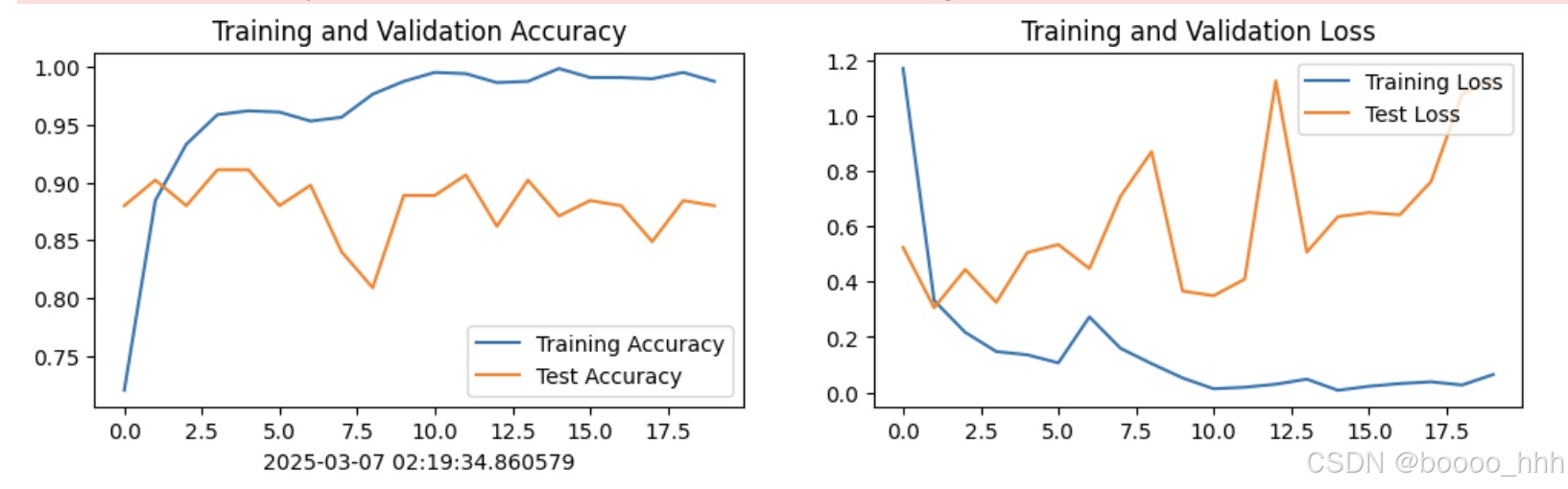
2. 模型评估
best_model.eval()
epoch_test_acc, epoch_test_loss = test(test_dl, best_model, loss_fn)
epoch_test_acc, epoch_test_loss(0.9111111111111111, 0.6467584735704198)
# 查看是否与我们记录的最高准确率一致
epoch_test_acc
0.9111111111111111
五、总结
初步学习了YOLOv5算法中的C3模块搭建网络,yolo5小且快,优化器的选择也很重要