matlab示例
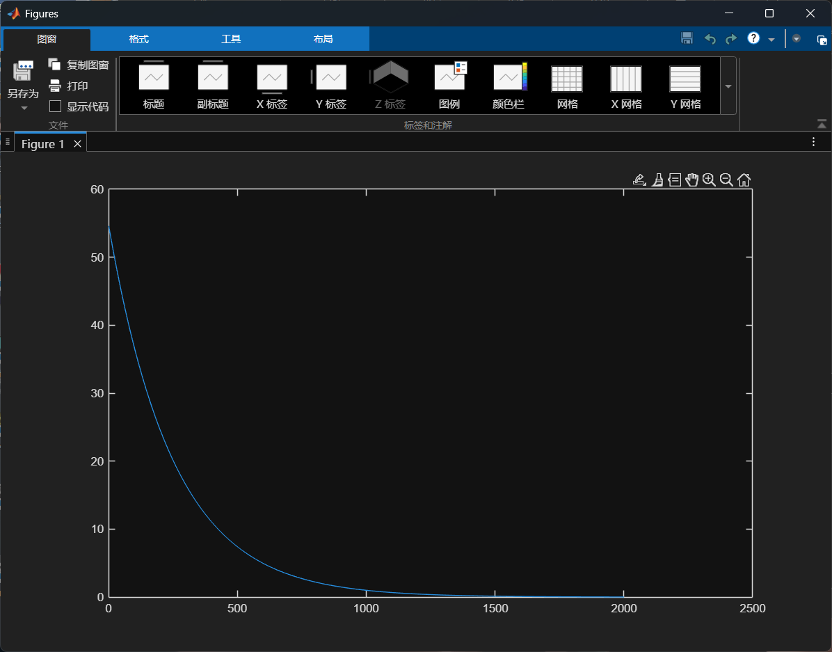
1.指数函数
clear all;
close all;
t=-10:0.01:10;
A=1;
a=-0.4;
ft=A*exp(a*t);
plot(t,ft);%plot为连续图,stem为离散图
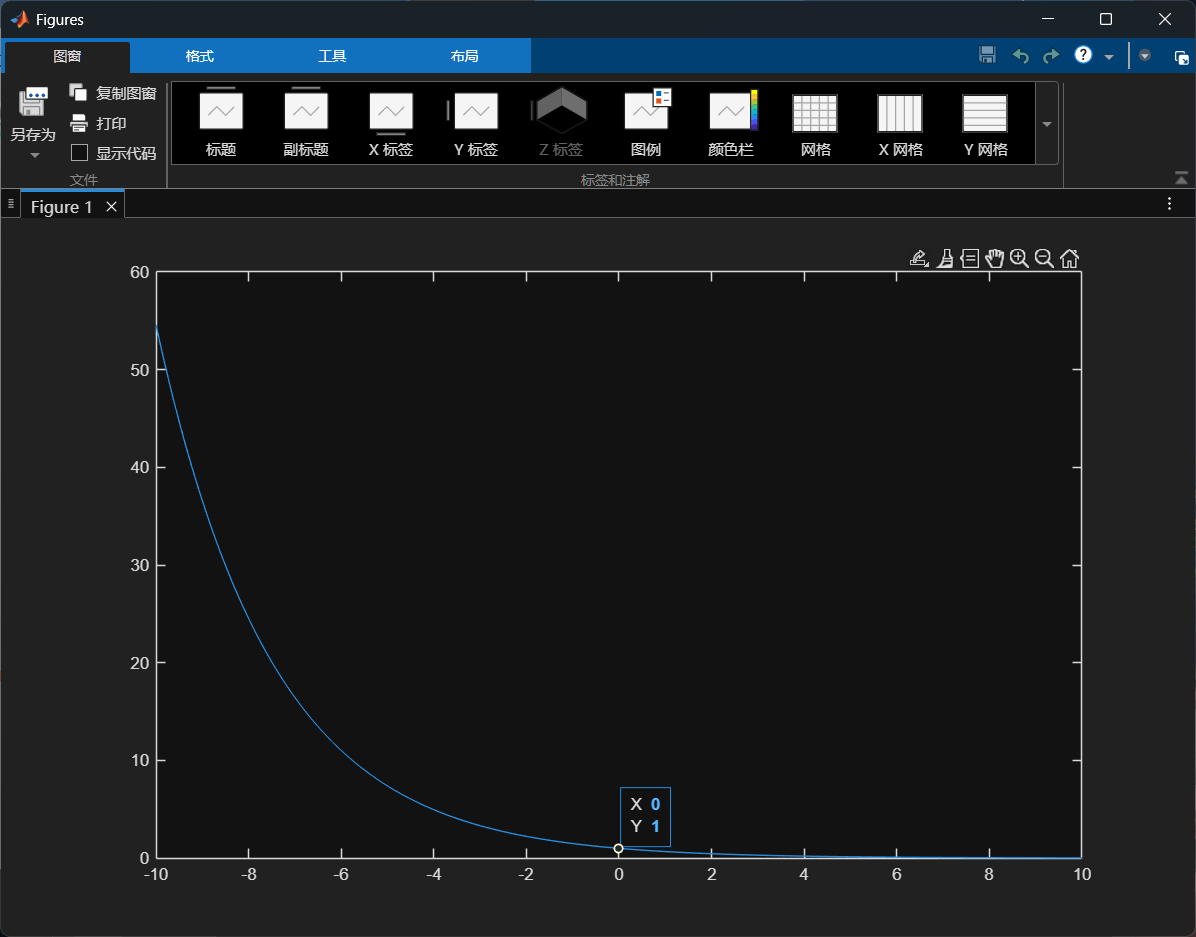
最后的plot如果改成plot(ft);则图形会自动确定x轴的范围。
2.三角函数波形
clear all;
close all;
t=-3:0.01:3;
ft=tripuls(t,4,0.5);%y = tripuls(t, width, skew),skew:斜率参数,控制三角波的偏斜程度
plot(t,ft);
ft1=tripuls(t,4,1);
figure,plot(t,ft1);%再创建一个窗口,如果没有,结果就只有一个图
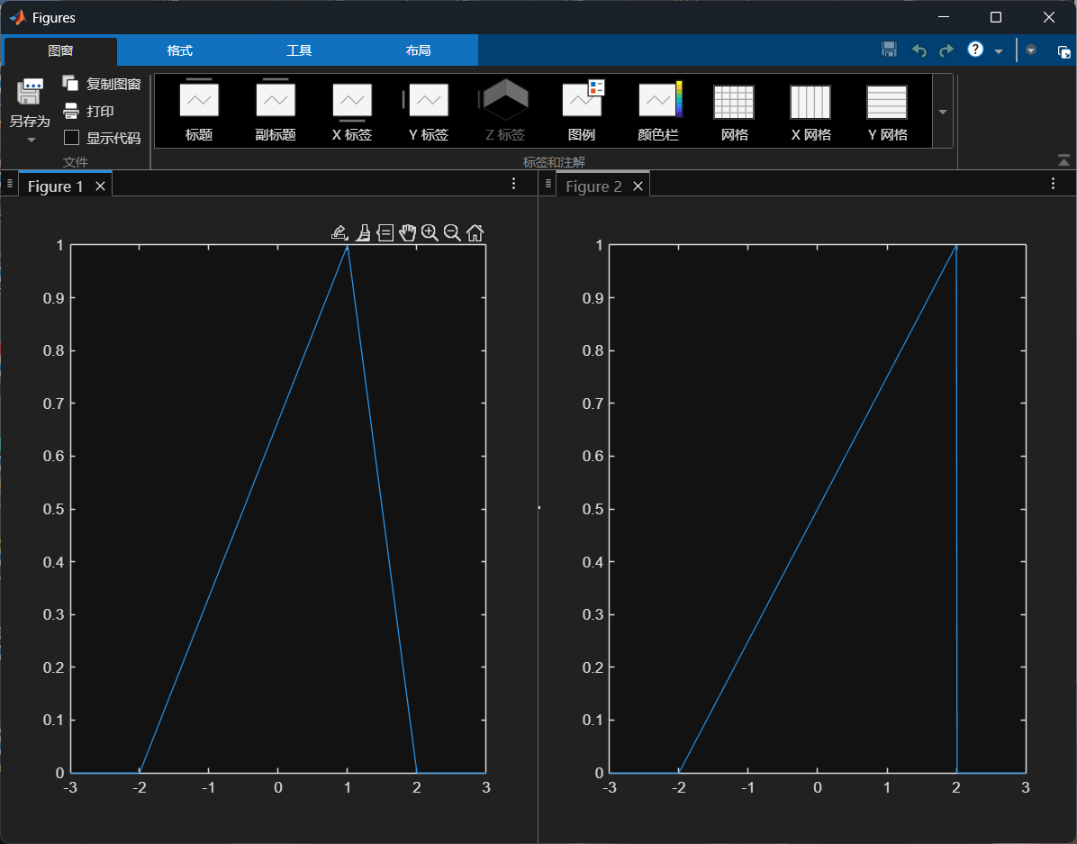
skew:偏斜度 = 三阶中心矩 / 标准差的三次方
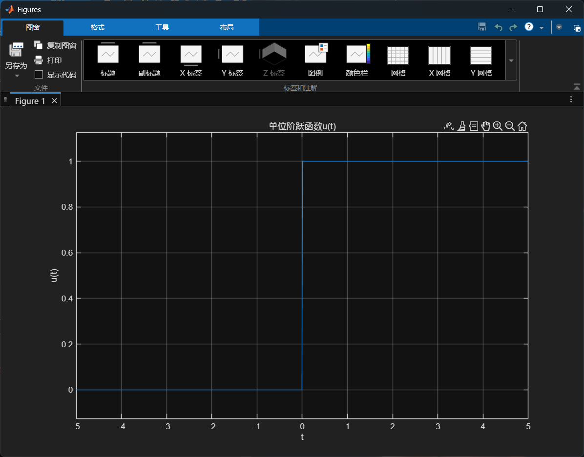
3.单位阶跃函数u(t)
% 定义符号变量t,用于后续符号计算
syms t
% 创建单位阶跃函数u(t),使用heaviside函数实现
u = heaviside(t);
% 绘制单位阶跃函数在区间[-5,5]上的图像
ezplot(u, [-5, 5]);%显函数、隐函数及参数方程
% 在图像中添加网格线
grid on;
% 为x轴添加标签,表示时间变量t
xlabel('t');
% 为y轴添加标签,表示函数值u(t)
ylabel('u(t)');
% 为图像添加标题,说明绘制的是单位阶跃函数
title('单位阶跃函数u(t)');
% 清除所有变量和关闭所有图形窗口
clear all;
close all;
% 定义时间范围
t = -2:0.01:5;
% 定义单位阶跃函数 u(t)
u_t = t >= 0;
plot(t,u_t)
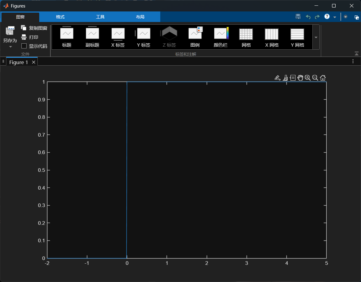
在 MATLAB 中,u_t = t >= 0; 的作用是定义一个单位阶跃函数 u(t)u(t) 。具体来说:
t是一个时间向量,包含了从 -2 到 5 的值,步长为 0.01。- 表达式
t >= 0对于每个元素t(i)返回一个逻辑值(布尔值),如果t(i)大于或等于 0,则返回true(在 MATLAB 中表示为 1),否则返回false(在 MATLAB 中表示为 0)。 - 因此,
u_t是一个与t同长度的逻辑数组,其中每个元素对应于t中相应位置的时间点是否大于或等于 0。
u_t = t >= 0;t >=0是一个判断,如果t确实大于等于0则返回true(1),反之则返回false(0)
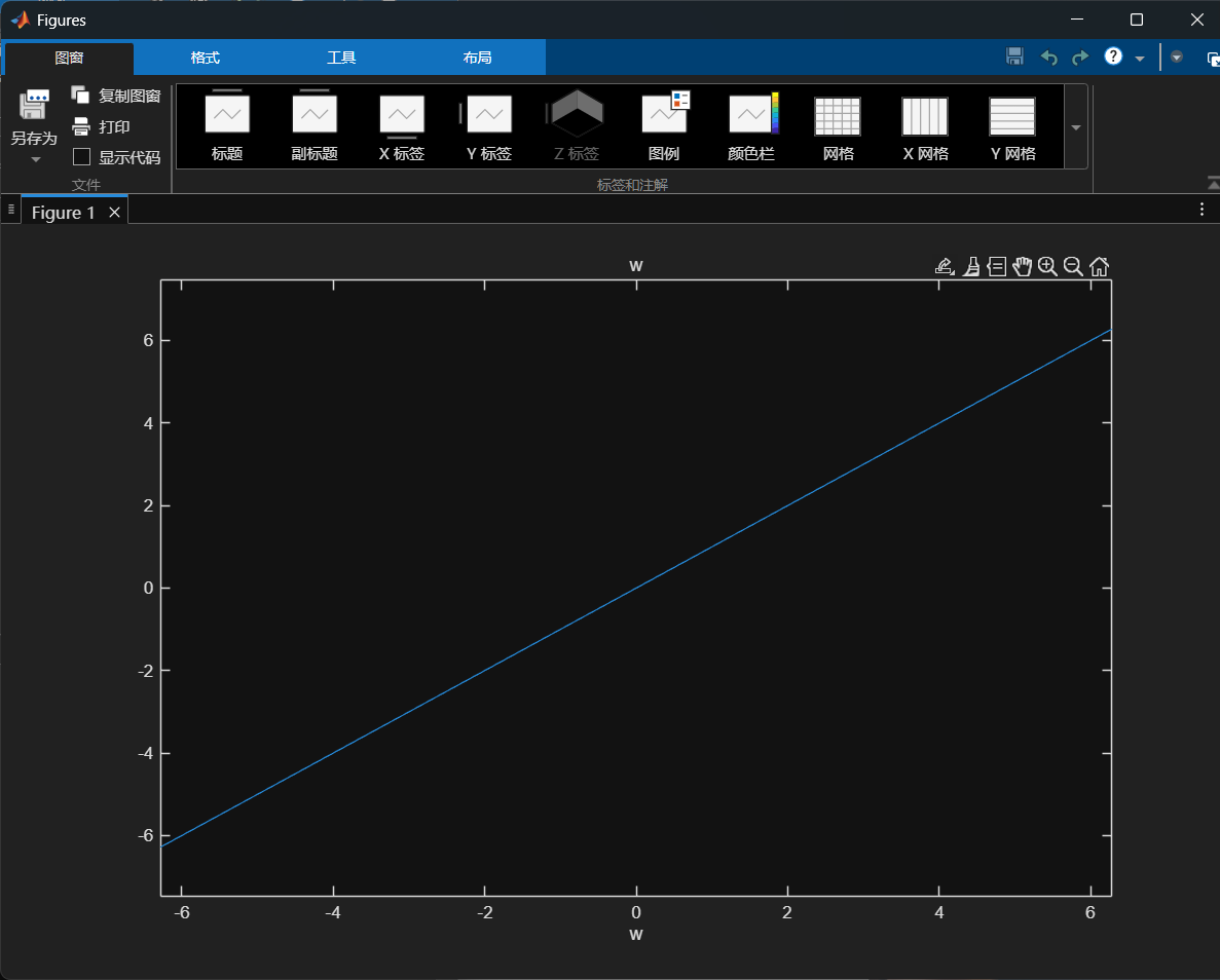
4.求下列函数的傅里叶变换
① sin2(2t)
% 清除所有变量和关闭所有图形窗口
clear all;
close all;
% 定义符号变量
syms t w
% 定义函数 f(t) = sin^2(2t)
f_t = sin(2*t)^2;
% 计算傅里叶变换 F(w)
F_w = fourier(f_t, t, w);
ezplot(w);
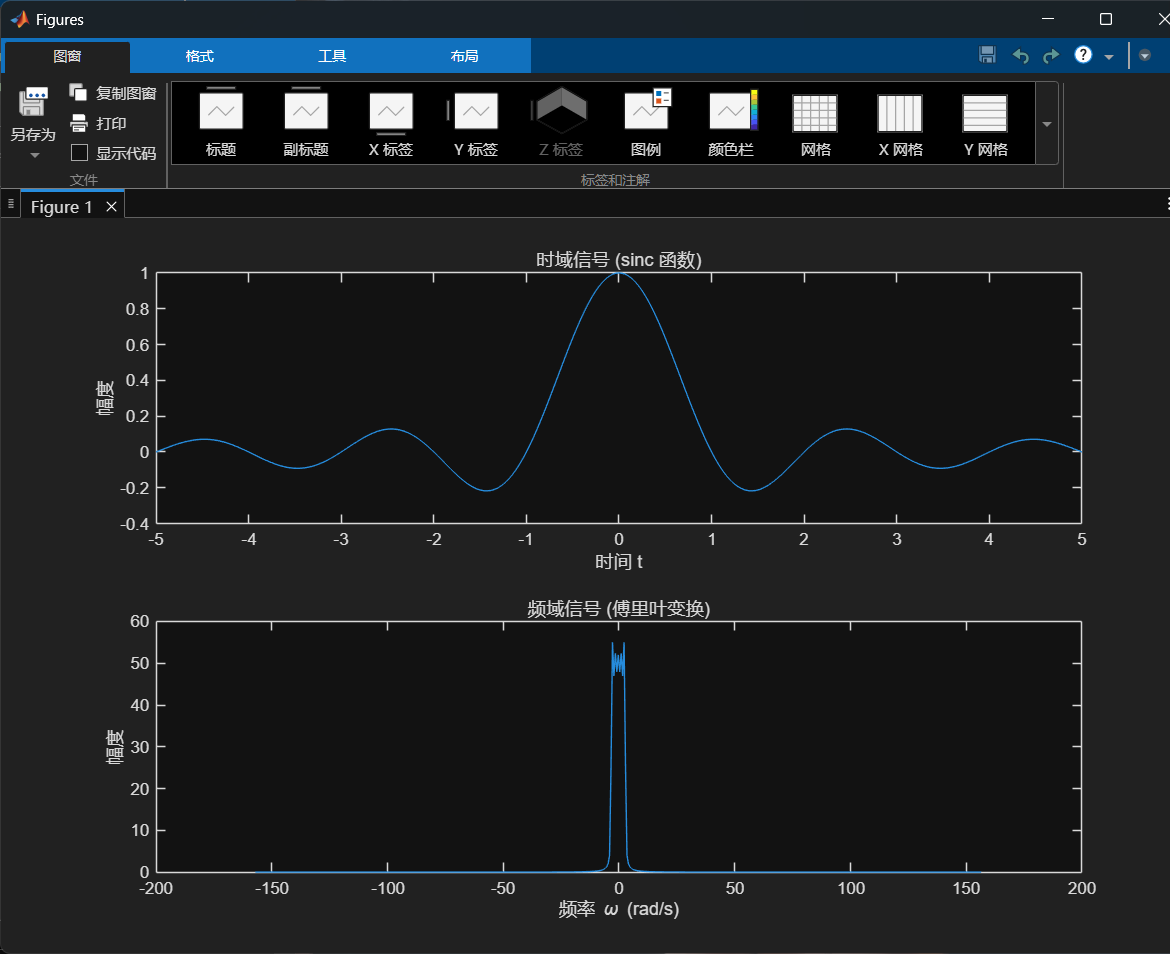
5.求下列信号的频谱图
④ sint/t
% 清除所有变量和关闭所有图形窗口
clear all;
close all;
% 参数设置
r = 0.02; % 时间步长
t = -5:r:5; % 时间向量
N = length(t); % 样本数量
% 创建 sinc 函数
f = sin(pi * t) ./ (pi * t);
f(isnan(f)) = 1; % 处理 t=0 的情况,sinc(0) = 1
% 计算傅里叶变换
F = fftshift(fft(f));
% 频率向量
w = (-N/2:N/2-1) * (2*pi / (N*r));
% 绘制原始信号
figure;
subplot(2,1,1);
plot(t, f);
title('时域信号 (sinc 函数)');
xlabel('时间 t');
ylabel('幅度');
% 绘制傅里叶变换结果
subplot(2,1,2);
plot(w, abs(F));
title('频域信号 (傅里叶变换)');
xlabel('频率 \omega (rad/s)');
ylabel('幅度');
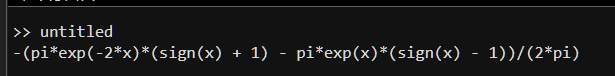
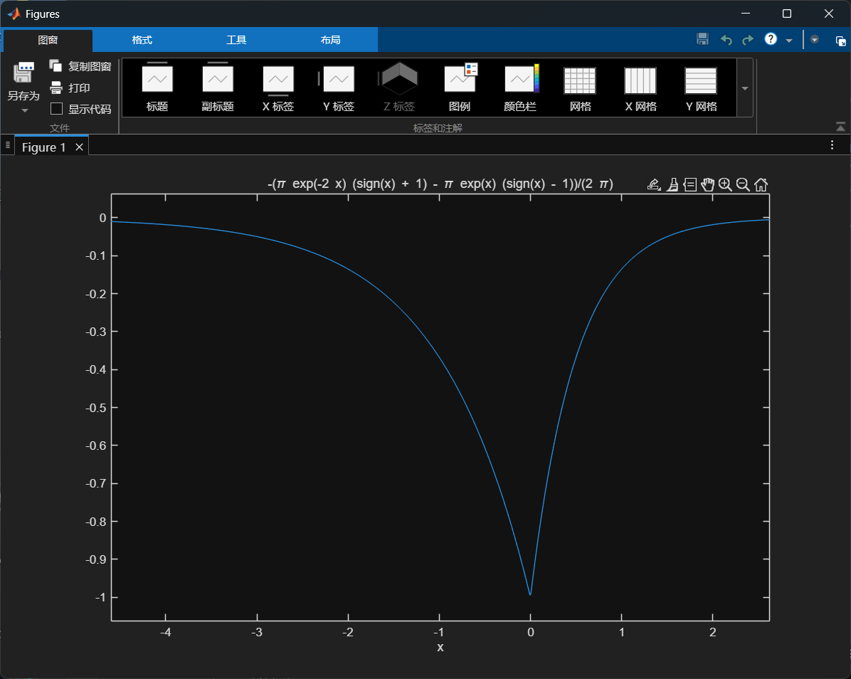
5.傅里叶反转
clear all;
syms t w;
f=ifourier(3/(-w^2+j*w-2));
ezplot(f);
disp(f);
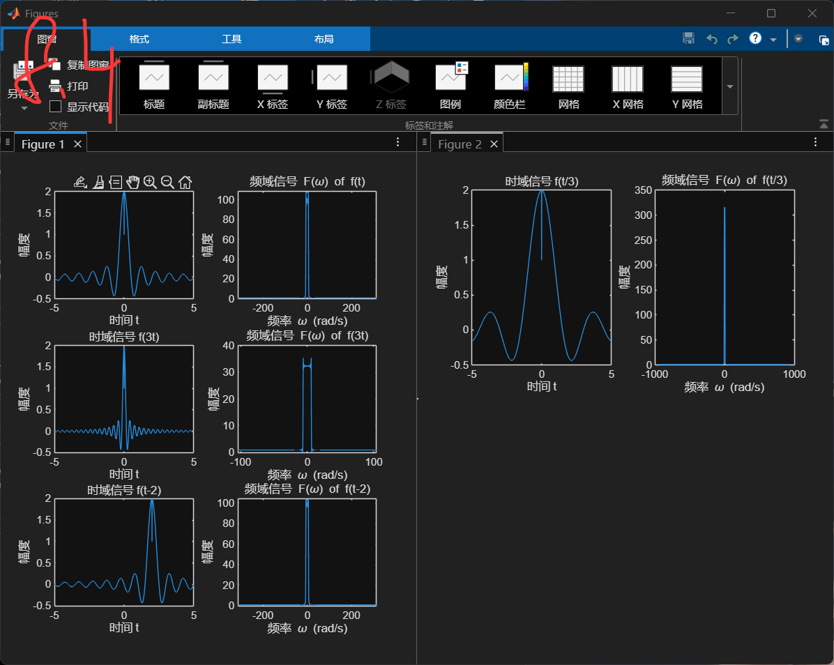
6.已知f(t)=sin(2πt)/πt,求f(3t)、f(t-2)、f(t/3)的频谱图
% 清除所有变量和关闭所有图形窗口
clear all;
close all;
% 参数设置
r = 0.01; % 时间步长
t = -5:r:5; % 时间向量
N = length(t); % 样本数量
% 创建 sinc 函数 f(t) = sin(2*pi*t) / (pi*t)
f_t = sin(2*pi*t) ./ (pi*t);
f_t(isnan(f_t)) = 1; % 处理 t=0 的情况,sinc(0) = 1
% 计算 f(t) 的傅里叶变换
F_t = fftshift(fft(f_t));
w_t = (-N/2:N/2-1) * (2*pi / (N*r));
% 创建 f(3t)
f_3t = sin(2*pi*(3*t)) ./ (pi*(3*t));
f_3t(isnan(f_3t)) = 1; % 处理 t=0 的情况,sinc(0) = 1
% 计算 f(3t) 的傅里叶变换
F_3t = fftshift(fft(f_3t));
w_3t = w_t / 3; % 频率缩放
% 创建 f(t-2)
f_t_minus_2 = sin(2*pi*(t-2)) ./ (pi*(t-2));
f_t_minus_2(isnan(f_t_minus_2)) = 1; % 处理 t=2 的情况,sinc(0) = 1
% 计算 f(t-2) 的傅里叶变换
F_t_minus_2 = fftshift(fft(f_t_minus_2));
w_t_minus_2 = w_t; % 频率不变
% 创建 f(t/3)
f_t_div_3 = sin(2*pi*(t/3)) ./ (pi*(t/3));
f_t_div_3(isnan(f_t_div_3)) = 1; % 处理 t=0 的情况,sinc(0) = 1
% 计算 f(t/3) 的傅里叶变换
F_t_div_3 = fftshift(fft(f_t_div_3));
w_t_div_3 = w_t * 3; % 频率缩放
% 绘制原始信号及其频谱图
figure;
subplot(3,2,1);
plot(t, f_t);
title('时域信号 f(t)');
xlabel('时间 t');
ylabel('幅度');
subplot(3,2,2);
plot(w_t, abs(F_t));
title('频域信号 F(\omega) of f(t)');
xlabel('频率 \omega (rad/s)');
ylabel('幅度');
% 绘制 f(3t) 及其频谱图
subplot(3,2,3);
plot(t, f_3t);
title('时域信号 f(3t)');
xlabel('时间 t');
ylabel('幅度');
subplot(3,2,4);
plot(w_3t, abs(F_3t));
title('频域信号 F(\omega) of f(3t)');
xlabel('频率 \omega (rad/s)');
ylabel('幅度');
% 绘制 f(t-2) 及其频谱图
subplot(3,2,5);
plot(t, f_t_minus_2);
title('时域信号 f(t-2)');
xlabel('时间 t');
ylabel('幅度');
subplot(3,2,6);
plot(w_t_minus_2, abs(F_t_minus_2));
title('频域信号 F(\omega) of f(t-2)');
xlabel('频率 \omega (rad/s)');
ylabel('幅度');
% 绘制 f(t/3) 及其频谱图
figure;
subplot(2,2,1);
plot(t, f_t_div_3);
title('时域信号 f(t/3)');
xlabel('时间 t');
ylabel('幅度');
subplot(2,2,2);
plot(w_t_div_3, abs(F_t_div_3));
title('频域信号 F(\omega) of f(t/3)');
xlabel('频率 \omega (rad/s)');
ylabel('幅度');