当前位置：首页 > news >正文

如何快速进行时间序列模型复现（以LSTM进行股票预测为例）

news 2025/10/28 6:34:50

写在前面

阅读完本文，你将

🎓 1. 在 1 小时内跑通第一个时间序列模型 (LSTM)。
🧰 2. 按照下面步骤，配置完环境、下载数据之后，直接运行start_demo.py 或将所有的代码复制到一个文件下运行即可直接完成复现。
😃 3. 得到一个适用于任何模型的股票预测模型复现模版。

前提

需要读者掌握conda命令和pip包管理工具，具有一定debug或使用AI进行Python代码debug的能力。

时序序列预测任务

在正式进入模型复现之前，我们需要知道我们在做什么，快速了解我们的时序序列预测任务，可以帮助我们快速上手论文复现。

时序序列预测任务，即训练出来模型的任务，总体可以表述为：考虑 $L$ 时间步的滑动窗口，每个滑动窗口时间步有 $D$ 个特征，我们要预测未来 $n$ 个时间步的某个指标的值。这里的描述有点抽象，此处以单只的股票预测为例。股票预测任务可以表述为，给定一只股票 $10$ 天的连续股票数据，每天股票数据特征包括开盘价、最高价、最低价、收盘价共 $4$ 个特征，我们要预测未来 $3$ 天的收盘价。此处 $L = 10, D = 4, n = 3$ 。于是我们模型的运作机制可以理解为给定 $\times D$ 的时间序列作为输入，输出为 $\times n$ 的预测值。

整个代码的任务

基于上面的内容，我们知道了整个时序预测任务是怎样的，但是这并不完整。我们的股票数据集通常并不是简单的滑动窗口时间步与特征数的乘积 $\times D$ ，而是一只股票所有时间的步数与特征数的乘积，即 $\times D$ ， $T$ 为一只股票的所有时间步。所以我们整个代码的任务为给定一个股票数据文件，我们将全部的数据读取，并进行切割，分成若干 $\times D$ 的训练数据，训练出一个模型，再用这个模型预测测试集的数据，然后分析预测结果的各类指标来评判模型的优劣，然后画出预测图像，再保存指标结果。

准备工作

🧰 一、环境配置

本内容的环境统一使用以下配置，方便统一复现。推荐使用conda配置环境。具体如下

# 安装 Python
conda create -n starter_demo python=3.11
conda activate starter_demo
# 安装 PyTorch
pip install torch==2.5.1 torchvision==0.20.1 torchaudio==2.5.1 --index-url https://download.pytorch.org/whl/cu124

📥 下载 demo 包 start_demo.zip

starter_demo.zip

starter_demo/
├── start_demo.py
├── requirements.txt
├── byd_data.csv

下载后解压，然后安装 requirements.txt 依赖，即在 start_demo/ 目录下运行命令

pip install -r requirements.txt

😃 二、数据集

本案例使用股票数据集，数据集为比亚迪（sz.002594）股票数据。输入数据部分内容和格式如下所示：

date	code	open	high	low	close	preclose	volume	amount	pctChg
2011/6/30	sz.002594	22	26.19	22	25.45	18	56292534	1.35E+09	41.38889
2011/7/1	sz.002594	25.77	28	25	28	25.45	33561279	8.99E+08	10.0196
2011/7/4	sz.002594	28.88	30.8	28.58	30.8	28	21964591	6.54E+08	10
2011/7/5	sz.002594	32.78	33.88	31.89	33.05	30.8	38108083	1.26E+09	7.3052
2011/7/6	sz.002594	32.8	35.55	32.11	33.4	33.05	31296719	1.06E+09	1.059

代码模板案例解析

整个案例的代码任务就是给定 $\times D_{input}$ 的csv文件输入，时序序列预测任务为，给定滑动窗口 $L = 10$ ，预测下一天的股价，即 $n = 1$ 。我们现在来看代码解析。

深度学习第一步通常是导入相关的包。

import torch
import torch.nn as nn
import torch.optim as optim
from torch.optim.lr_scheduler import ReduceLROnPlateau
from torch.utils.data import Dataset, DataLoader
import pandas as pd
import numpy as np # numpy==1.23.5
from sklearn.preprocessing import MinMaxScaler
from sklearn.metrics import mean_squared_error, mean_absolute_error, r2_score
import matplotlib.pyplot as plt
import random

然后我们进入整个代码的任务。

设定随机种子与训练设备

设计随机种子可以让多次运行都有相同的结果。训练设备可以使用cpu或者cuda。

# Set random seed
torch.manual_seed(42)
np.random.seed(42)
random.seed(42)# Device
device = torch.device("cuda" if torch.cuda.is_available() else "cpu")
print(f'Using device: {device}')

数据预处理

数据预处理主要工作就是导入数据，设定我们的输入和输出是什么，随后按照我们的要求进行划分数据，最后设定训练集、验证集（可选）和测试集。例如此处我们导入股票数据，输入就是除了收盘价以外的特征，滑动窗口为10，输出就是收盘价。最后我们将训练集、验证集和测试集以8:1:1的比例进行划分。

# Load data
df = pd.read_csv('byd_data.csv')
df['date'] = pd.to_datetime(df['date'])
df['timestamp'] = df['date'].astype(np.int64) // 10**9  # Convert date to numeric timestamp# 特征字段
x_features = ['timestamp', 'open', 'high', 'low', 'preclose', 'volume', 'amount', 'pctChg']  # 不含 close
y_feature = 'close'# 提取原始特征和目标
X_raw = df[x_features].values
y_raw = df[y_feature].values.reshape(-1, 1)# 滑动窗口构造函数，x 和 y 分开处理
def create_sequences_split(X, y, seq_length=10):xs, ys = [], []for i in range(len(X) - seq_length):x_seq = X[i:i+seq_length, :]       # (L, D)y_target = y[i+seq_length, 0]      # scalarxs.append(x_seq)ys.append(y_target)return np.array(xs), np.array(ys)seq_length = 10
X_all, y_all = create_sequences_split(X_raw, y_raw, seq_length)# 划分训练、验证、测试
total = len(X_all)
train_end = int(total * 0.8)
val_end = int(total * 0.9)X_train_raw, y_train_raw = X_all[:train_end], y_all[:train_end]
X_val_raw, y_val_raw = X_all[train_end:val_end], y_all[train_end:val_end]
X_test_raw, y_test_raw = X_all[val_end:], y_all[val_end:]

数据归一化

随后进行数据归一化，数据归一化的目的是为了加速运算。想象一下我们的数据集，若在数值上的取值范围为[-10000,10000]，那么在计算机运算时，效率会十分低下。若将其压缩到[-1,1]，则可以大大提升计算效率。此外，归一化必须避开测试集和验证集，防止数据泄漏。

# 分别归一化 X 和 y
# 输入特征 scaler：用训练集拟合
scaler_x = MinMaxScaler()
X_train = scaler_x.fit_transform(X_train_raw.reshape(-1, X_train_raw.shape[-1])).reshape(X_train_raw.shape)
X_val = scaler_x.transform(X_val_raw.reshape(-1, X_val_raw.shape[-1])).reshape(X_val_raw.shape)
X_test = scaler_x.transform(X_test_raw.reshape(-1, X_test_raw.shape[-1])).reshape(X_test_raw.shape)# 目标值 scaler：只用 y_train 拟合，防止泄漏
scaler_y = MinMaxScaler()
y_train = scaler_y.fit_transform(y_train_raw.reshape(-1, 1)).reshape(-1)
y_val = scaler_y.transform(y_val_raw.reshape(-1, 1)).reshape(-1)
y_test = scaler_y.transform(y_test_raw.reshape(-1, 1)).reshape(-1)

制作数据加载器

有了切分好的数据还不够，我们需要制作适用于Pytorch框架的，能用用于数据训练格式的数据，这就是我们的数据加载器（DataLoader），具体来说就是用 torch.tensor 包装一下，然后传给专用的DataLoader。

# Dataset class
class StockDataset(Dataset):def __init__(self, X, y):self.X = torch.tensor(X, dtype=torch.float32)self.y = torch.tensor(y, dtype=torch.float32)def __len__(self):return len(self.X)def __getitem__(self, idx):return self.X[idx], self.y[idx]train_dataset = StockDataset(X_train, y_train)
val_dataset = StockDataset(X_val, y_val)
test_dataset = StockDataset(X_test, y_test)train_loader = DataLoader(train_dataset, batch_size=32, shuffle=True)
val_loader = DataLoader(val_dataset, batch_size=32, shuffle=False)
test_loader = DataLoader(test_dataset, batch_size=32, shuffle=False)

定义模型

随后我们需要定义我们的模型。模型代码部分如下：

# Model
class LSTM(nn.Module):def __init__(self, d_input, d_model=16):super().__init__()self.d_model = d_modelself.input_proj = nn.Linear(d_input, d_model)self.lstm = nn.LSTM(d_model, d_model)self.linear = nn.Linear(d_model, 1)def forward(self, x):# x: (B, L, d_input)x = self.input_proj(x) # (B, L, d_input) -> (B, L, D)B, L, D = x.shapeh0 = torch.zeros(1, L, D) # LSTM隐藏层c0 = torch.zeros(1, L, D) # LSTM当前状态单元out, _ = self.lstm(x,(h0, c0))  # (B, L, D)# 取最后时间步 → 映射为标量out = out[:, -1, :]  # (B, D)out = self.linear(out).squeeze(-1)  # (B,)return out

模型训练

然后我们搭建模型训练模版。

model = LSTM(d_input=8, d_model=16).to(device)
optimizer = optim.Adam(model.parameters(), lr=0.001)
criterion = nn.MSELoss()
scheduler = ReduceLROnPlateau(optimizer, mode='min', factor=0.1, patience=25)  # 学习率调整策略

训练模型

# Training
epochs = 30early_patience = 0.24
early_patience_epochs = int(early_patience * epochs)  # 早停耐心值（转换为epoch数）
best_val_loss = float('inf')  # 初始化最佳验证集损失
early_stop_counter = 0  # 早停计数器for epoch in range(epochs):model.train()train_loss = 0for batch_x, batch_y in train_loader:batch_x, batch_y = batch_x.to(device), batch_y.to(device)optimizer.zero_grad()output = model(batch_x)loss = criterion(output, batch_y)loss.backward()optimizer.step()train_loss += loss.item()if epoch % 10 == 0:print(f'Epoch {epoch+1}/{epochs}, Train Loss: {train_loss / len(train_loader)}')# Valmodel.eval()val_loss = 0with torch.no_grad():for batch_x, batch_y in val_loader:batch_x, batch_y = batch_x.to(device), batch_y.to(device)output = model(batch_x)loss = criterion(output, batch_y)val_loss += loss.item()avg_val_loss = val_loss / len(val_loader)  # 计算本epoch的平均验证损失scheduler.step(avg_val_loss)  # 更新学习率（基于当前验证损失）if epoch % 10 == 0:print(f'Val Loss: {val_loss / len(val_loader)}')# 早停判断if avg_val_loss < best_val_loss:best_val_loss = avg_val_lossearly_stop_counter = 0  # 重置早停计数器# TODO: 保存最优模型else:early_stop_counter += 1if early_stop_counter >= early_patience_epochs:print(f'Early stopping triggered at epoch {epoch + 1}.')break  # 早停

模型评估

# Evaluation
def evaluate(loader, model, scaler, dataset_name):model.eval()preds, trues = [], []with torch.no_grad():for batch_x, batch_y in loader:batch_x = batch_x.to(device)output = model(batch_x)preds.extend(output.cpu().numpy())trues.extend(batch_y.cpu().numpy())preds = np.array(preds)trues = np.array(trues)# Inverse scale (only for close)preds = scaler.inverse_transform(preds.reshape(-1, 1))[:, 0]trues = scaler.inverse_transform(trues.reshape(-1, 1))[:, 0]mse = mean_squared_error(trues, preds)mae = mean_absolute_error(trues, preds)rmse = np.sqrt(mse)mape = np.mean(np.abs((trues - preds) / trues)) * 100 if np.all(trues != 0) else float('inf')r2 = r2_score(trues, preds)print(f'{dataset_name} Metrics: MSE={mse}, MAE={mae}, RMSE={rmse}, MAPE={mape}, R2={r2}')return preds, trues, {'MSE': mse, 'MAE': mae, 'RMSE': rmse, 'MAPE': mape, 'R2': r2}# Evaluate on alltrain_preds, train_trues, train_metrics = evaluate(train_loader, model, scaler_y, 'Train')
val_preds, val_trues, val_metrics = evaluate(val_loader, model, scaler_y, 'Val')
test_preds, test_trues, test_metrics = evaluate(test_loader, model, scaler_y, 'Test')

保存结果

# Save metrics
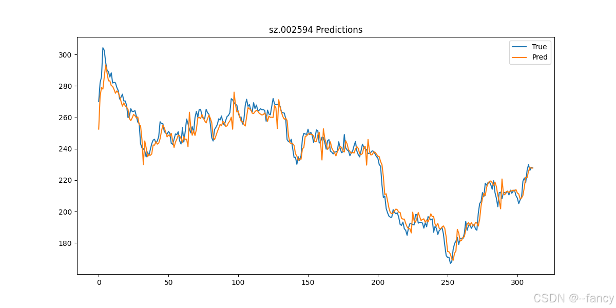
with open('metrics.txt', 'w') as f:f.write(f'Train: {train_metrics}\nVal: {val_metrics}\nTest: {test_metrics}\n')# Visualization (test set)
plt.figure(figsize=(12, 6))
plt.plot(test_trues, label='True')
plt.plot(test_preds, label='Pred')
plt.legend()
plt.title('sz.002594 Predictions')
plt.savefig('prediction.png')
plt.show()# Rolling window validation (on val set, example with window size)
print('Rolling window validation on val...')
# Implement rolling: for simplicity, re-evaluate val as is; extend if needed.

如何运行

📊 一、如何运行第一个模型

直接运行 starter_demo.py 该demo展示了使用LSTM模型进行股票时间序列预测，用比亚迪股票（sz.002594）连续的 10 天数据预测第 11 天的收盘价 close。

🧠 二、输出结果解读

若成功运行 starter_demo.py ，则会出现下面类似内容！

Using device: cpu/cuda
Epoch 1/30, Train Loss: 0.020305860580172006
Val Loss: 0.04599916897714138
Epoch 11/30, Train Loss: 0.00015859248049729594
Val Loss: 0.0013557001890148967
Early stopping triggered at epoch 14.
Train Metrics: MSE=12.37447452545166, MAE=2.015416383743286, RMSE=3.5177371313746084, MAPE=3.4971337765455246, R2=0.9956204295158386
Val Metrics: MSE=132.31785583496094, MAE=8.793128967285156, RMSE=11.502949875356363, MAPE=3.040638193488121, R2=0.8819977045059204
Test Metrics: MSE=31.45413589477539, MAE=4.196530818939209, RMSE=5.608398692565944, MAPE=1.7993846908211708, R2=0.9653774499893188
Rolling window validation on val...

此外，代码运行结束之后，还保存了两个额外的结果文件 metrics.txt和 prediction.png 分别存放了评价指标结果（用于实验结果展示）和预测值与真实值的结果（用于画图展示预测结果）。显示预测结果如下图所示。

在这里插入图片描述