Tanh 函数详解

Tanh 函数详解

1. 基本概念

Tanh 函数（双曲正切函数）是深度学习和神经网络中常用的激活函数之一。它是双曲函数家族中的一员，与传统的三角函数类似但定义在双曲几何中。

2. 数学定义

2.1 基本公式

Tanh 函数的定义基于指数函数：

$$\tanh (x)=\frac{\sinh (x)}{\cosh (x)}=\frac{e^x-e^{-x}}{e^x+e^{-x}}$$

也可以表示为：

$$\tanh (x)=\frac{e^{2x}-1}{e^{2x}+1}=1-\frac{2}{e^{2x}+1}$$

2.2 导数公式

Tanh 函数的导数为：

$$\frac{d}{dx}\tanh (x)=1-{\tanh }^2(x)$$

证明过程：
$$\frac{d}{dx}\tanh (x)=\frac{d}{dx}\left(\frac{e^x-e^{-x}}{e^x+e^{-x}}\right)=\frac{(e^x+e^{-x}{)}^2-(e^x-e^{-x}{)}^2}{(e^x+e^{-x}{)}^2}=1-{\left(\frac{e^x-e^{-x}}{e^x+e^{-x}}\right)}^2=1-{\tanh }^2(x)$$

3. 特性分析

3.1 函数特性

• 值域：(-1, 1)
• 定义域：(-∞, +∞)
• 奇函数：tanh(-x) = -tanh(x)
• 在原点：tanh(0) = 0
• 渐近线：当 x → +∞ 时，tanh(x) → 1；当 x → -∞ 时，tanh(x) → -1

3.2 与 Sigmoid 函数的关系

$$\tanh (x)=2\sigma (2x)-1$$
其中 σ(x) 是 Sigmoid 函数：σ(x) = 1/(1+e^{-x})

4. Python 实现与可视化

import numpy as np
import matplotlib.pyplot as plt
import seaborn as sns# 设置中文字体和样式
plt.rcParams['font.sans-serif'] = ['SimHei']
plt.rcParams['axes.unicode_minus'] = False
sns.set_style("whitegrid")def tanh(x):"""Tanh 函数实现"""return np.tanh(x)def tanh_derivative(x):"""Tanh 函数导数实现"""return 1 - np.tanh(x)**2# 创建数据点
x = np.linspace(-5, 5, 1000)
y_tanh = tanh(x)
y_derivative = tanh_derivative(x)# 创建图形
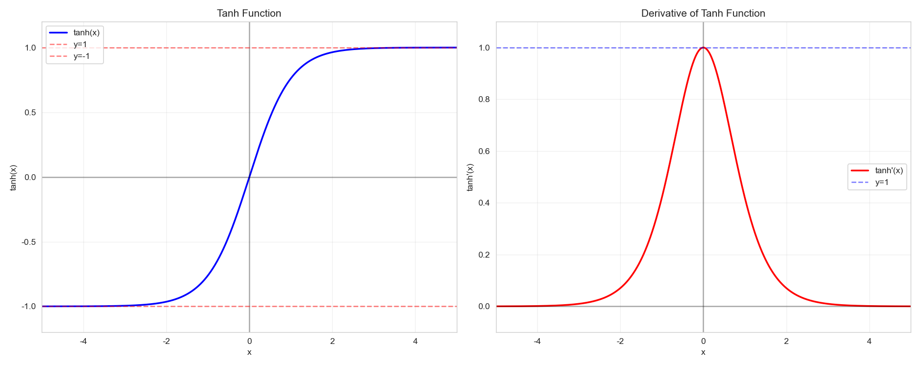
fig, (ax1, ax2) = plt.subplots(1, 2, figsize=(15, 6))# 绘制 Tanh 函数
ax1.plot(x, y_tanh, 'b-', linewidth=2, label='tanh(x)')
ax1.axhline(y=0, color='k', linestyle='-', alpha=0.3)
ax1.axvline(x=0, color='k', linestyle='-', alpha=0.3)
ax1.axhline(y=1, color='r', linestyle='--', alpha=0.5, label='y=1')
ax1.axhline(y=-1, color='r', linestyle='--', alpha=0.5, label='y=-1')
ax1.set_xlabel('x')
ax1.set_ylabel('tanh(x)')
ax1.set_title('Tanh 函数')
ax1.legend()
ax1.grid(True, alpha=0.3)
ax1.set_xlim(-5, 5)
ax1.set_ylim(-1.2, 1.2)# 绘制 Tanh 导数
ax2.plot(x, y_derivative, 'r-', linewidth=2, label="tanh'(x)")
ax2.axhline(y=0, color='k', linestyle='-', alpha=0.3)
ax2.axvline(x=0, color='k', linestyle='-', alpha=0.3)
ax2.axhline(y=1, color='b', linestyle='--', alpha=0.5, label='y=1')
ax2.set_xlabel('x')
ax2.set_ylabel("tanh'(x)")
ax2.set_title('Tanh 函数导数')
ax2.legend()
ax2.grid(True, alpha=0.3)
ax2.set_xlim(-5, 5)
ax2.set_ylim(-0.1, 1.1)plt.tight_layout()
plt.show()# 绘制对比图
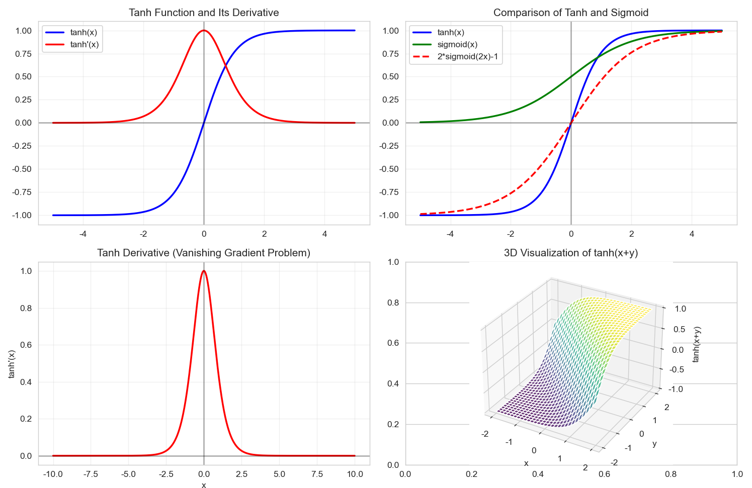
plt.figure(figsize=(12, 8))plt.subplot(2, 2, 1)
plt.plot(x, y_tanh, 'b-', linewidth=2, label='tanh(x)')
plt.plot(x, y_derivative, 'r-', linewidth=2, label="tanh'(x)")
plt.axhline(y=0, color='k', linestyle='-', alpha=0.3)
plt.axvline(x=0, color='k', linestyle='-', alpha=0.3)
plt.title('Tanh 函数及其导数')
plt.legend()
plt.grid(True, alpha=0.3)plt.subplot(2, 2, 2)
# 与 Sigmoid 对比
sigmoid = 1 / (1 + np.exp(-x))
sigmoid_scaled = 2 * sigmoid - 1
plt.plot(x, y_tanh, 'b-', linewidth=2, label='tanh(x)')
plt.plot(x, sigmoid, 'g-', linewidth=2, label='sigmoid(x)')
plt.plot(x, sigmoid_scaled, 'r--', linewidth=2, label='2*sigmoid(2x)-1')
plt.axhline(y=0, color='k', linestyle='-', alpha=0.3)
plt.axvline(x=0, color='k', linestyle='-', alpha=0.3)
plt.title('Tanh 与 Sigmoid 对比')
plt.legend()
plt.grid(True, alpha=0.3)plt.subplot(2, 2, 3)
# 梯度消失问题演示
x_detailed = np.linspace(-10, 10, 1000)
y_tanh_detailed = tanh(x_detailed)
y_derivative_detailed = tanh_derivative(x_detailed)
plt.plot(x_detailed, y_derivative_detailed, 'r-', linewidth=2)
plt.axhline(y=0, color='k', linestyle='-', alpha=0.3)
plt.axvline(x=0, color='k', linestyle='-', alpha=0.3)
plt.title('Tanh 导数（梯度消失问题）')
plt.xlabel('x')
plt.ylabel("tanh'(x)")
plt.grid(True, alpha=0.3)plt.subplot(2, 2, 4)
# 3D 可视化准备
X, Y = np.meshgrid(np.linspace(-2, 2, 30), np.linspace(-2, 2, 30))
Z = tanh(X + Y)
from mpl_toolkits.mplot3d import Axes3D
ax = plt.subplot(2, 2, 4, projection='3d')
ax.plot_surface(X, Y, Z, cmap='viridis', alpha=0.8)
ax.set_title('tanh(x+y) 3D 可视化')
ax.set_xlabel('x')
ax.set_ylabel('y')
ax.set_zlabel('tanh(x+y)')plt.tight_layout()
plt.show()

5. 在深度学习中的应用

5.1 优点

1. 零中心化：输出以 0 为中心，有助于优化过程
2. 平滑梯度：导数连续且平滑
3. 有界输出：输出在 (-1, 1) 范围内，防止梯度爆炸

5.2 缺点

1. 梯度消失：当 |x| 较大时，梯度接近 0
2. 计算复杂度：涉及指数运算，计算成本较高

5.3 使用示例

import torch
import torch.nn as nn# 在 PyTorch 中使用 Tanh
class SimpleNN(nn.Module):def __init__(self):super(SimpleNN, self).__init__()self.fc1 = nn.Linear(10, 50)self.activation = nn.Tanh()self.fc2 = nn.Linear(50, 1)def forward(self, x):x = self.activation(self.fc1(x))x = self.fc2(x)return x# 在 NumPy 中手动实现
def tanh_manual(x):"""手动实现的 Tanh 函数"""return (np.exp(x) - np.exp(-x)) / (np.exp(x) + np.exp(-x))def tanh_derivative_manual(x):"""手动实现的 Tanh 导数"""tanh_x = tanh_manual(x)return 1 - tanh_x**2

6. 总结

Tanh 函数作为经典的激活函数，在深度学习发展初期被广泛使用。虽然现在 ReLU 及其变体更为流行，但 Tanh 在某些特定场景下仍有其价值，特别是在需要输出在 (-1, 1) 范围内的网络中。理解 Tanh 函数的数学特性和行为对于深入理解神经网络的工作原理非常重要。