【点云】point Transformer V1文章梳理

every blog every motto: You can do more than you think.
https://blog.csdn.net/weixin_39190382?type=blog

0. 前言

point Transformer有几个点：

1. 将Transformer引入到点云中（不确定之前是不是有人这么做）
2. 采用unet形式
3. 由于点云的特点，使用最远点采样+knn，获取局部点
4. 注意力机制方面的改进
   • 注意力和特征都加位置编码
   • 用”领域特征-中心点特征“作为权重（还要加上位置编码）
   • 权重部分还会经过一个MLP
5. transformer block采用残差连接

---

code: https://github.heygears.com/POSTECH-CVLab/point-transformer?tab=readme-ov-file

time: 2020.12.16

1. 正文

1.1 相关工作

1. 基于投影

将点云投影到二维平面，生成规则图像，然后使用 2D CNN 提取特征，再进行多视角融合。

TangentConv 将局部表面几何投影到切平面，生成切平面图像，用二维卷积处理，但依赖切平面估计。

缺点：投影会压缩几何信息，可能未充分利用点云稀疏性，平面选择和三维遮挡可能影响识别性能。

2. 基于体素

将点云体素化，再在三维网格上进行卷积。

优点：将不规则点云转化为规则表示，便于卷积操作。

缺点：分辨率增加时计算和内存开销大。

解决方案：利用稀疏性，如 OctNet 使用不平衡八叉树，稀疏卷积只计算非空体素【9,3】。

注意：体素化量化仍可能导致几何细节丢失。

3. 基于 point 的网络

直接处理嵌入连续空间的点云集合，无需量化或投影。

PointNet 使用排列不变操作（逐点 MLP + 池化）聚合集合特征。

PointNet++ 在层级空间结构中增加对局部几何布局的敏感性。

可结合高效采样策略，提高计算效率【27,7,46,50,11】。

4. 基于图

将点集构建成图，进行消息传递或图卷积：

DGCNN 在 kNN 图上进行图卷积

PointWeb 密集连接局部邻域

ECC 使用动态边条件卷积

SPG 使用超级点图表示上下文关系

KCNet 使用核相关 + 图池化

Wang 等研究局部谱图卷积

GACNet 使用图注意力卷积

HPEIN 构建层级点-边交互架构

DeepGCNs 探索图卷积深度在 3D 场景理解中的优势

5. 基于连续卷积

PCCN 将卷积核表示为 MLP

SpiderCNN 使用多项式函数族定义卷积核权重

Spherical CNN 解决 3D 旋转等变性

PointConv 和 KPConv 根据坐标构建卷积核

InterpCNN 使用坐标插值生成卷积权重

PointCNN 对无序点云重新排序

Ummenhofer 等将连续卷积应用于粒子流体动力学

6. Transformer

现有点云注意力方法多为全局注意力：

计算开销大

不适合大规模场景

使用标量点积，所有通道共享聚合权重

本文方法创新点：

在局部应用自注意力，使网络可扩展到百万点大场景

使用向量注意力，提高精度

强调位置编码的重要性，而先前方法通常忽略

1.2 背景

自注意力机制分为标量注意力机制，向量注意力机制。

标量注意力机制：

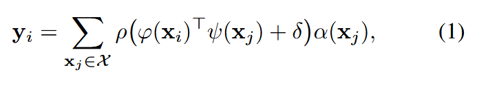
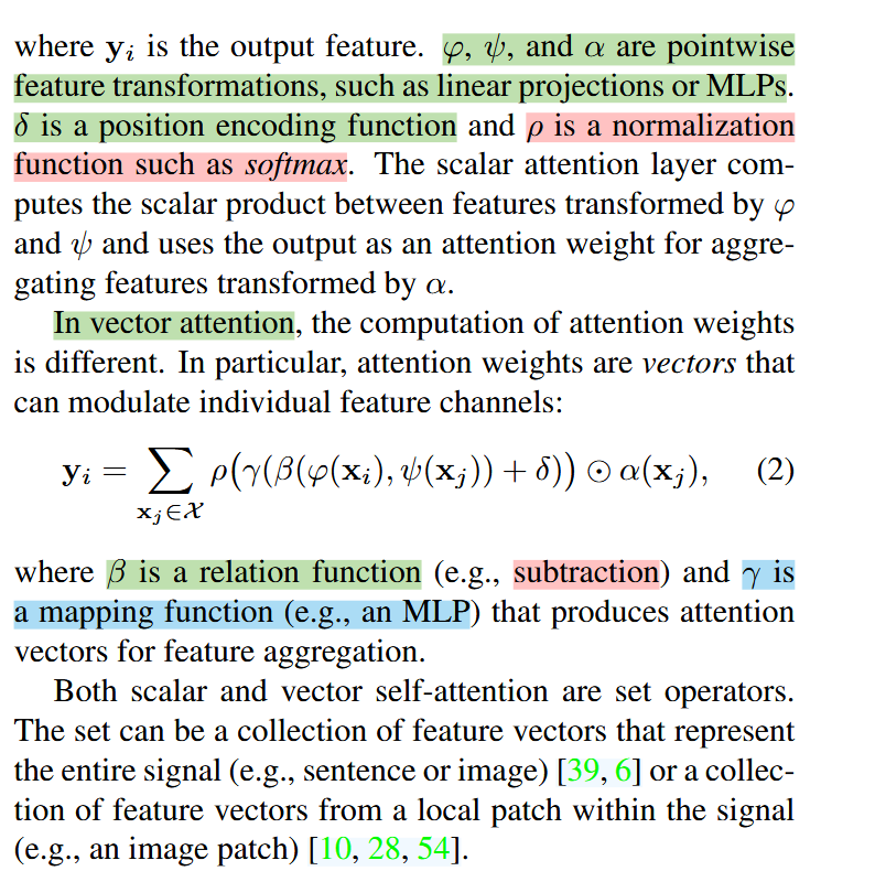
向量注意力机制

这两类自注意力算子本质上都是集合算子，既可以在整个集合上作用（如句子、整幅图像），也可以只在局部子集上作用（如图像 patch）。

1.3 point Transformer Layer

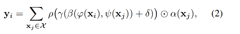
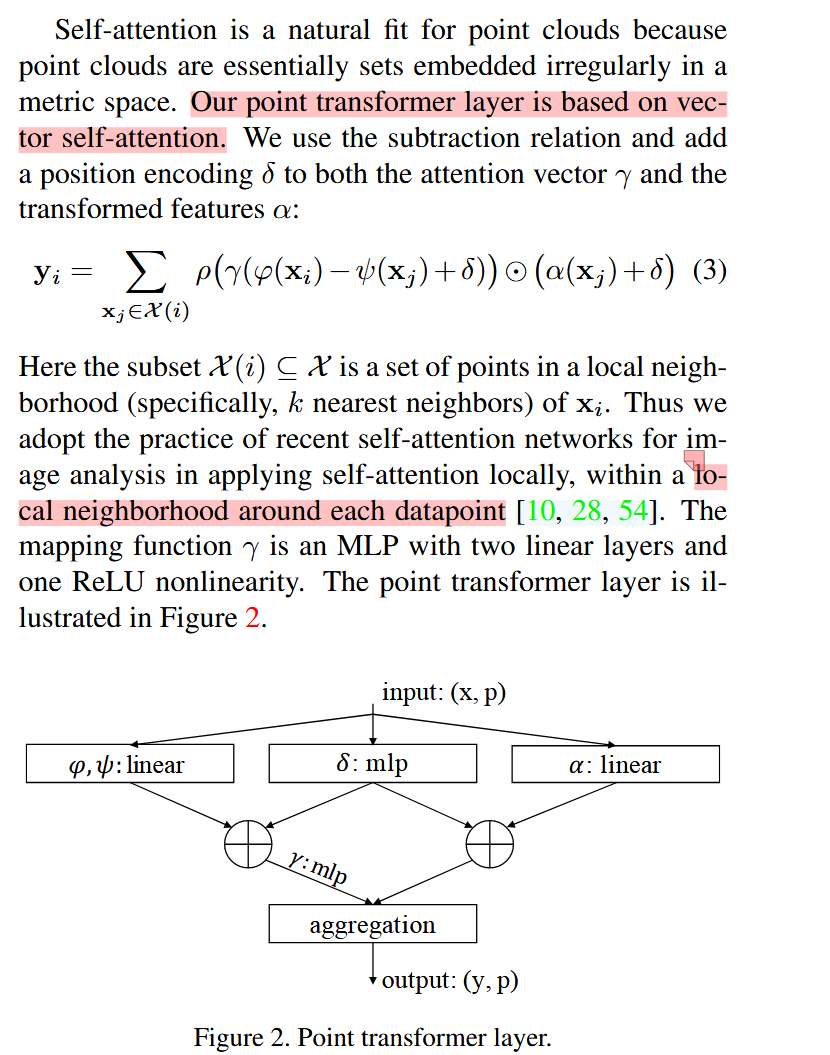
点云天然就是不规则的集合，因此自注意力特别适合点云。Point Transformer 层基于向量自注意力，采用减法关系并在注意力分支和特征分支都加入位置编码：

其中 $X^{(i)}$ 是 $x_i$ 的 $k$ 近邻集合**（局部邻域）**。映射函数 $\gamma$ 是一个两层线性层 + ReLU 的 MLP。结构如图 2 所示。

1.4 位置编码

位置编码让注意力能够感知局部空间结构。

• 在 NLP/图像中，常用正弦余弦或归一化坐标范围手工设计。

• 在 3D 点云中，点的坐标天然可用作位置编码。

本文提出 可训练的参数化位置编码：

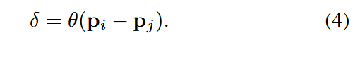
其中 $\theta$ 是一个两层线性层 + ReLU 的 MLP。

实验发现，位置编码对注意力生成分支和特征变换分支都很重要，因此在公式 (3) 的两个分支中都加了
$\delta$。 与整个网络一起端到端训练。

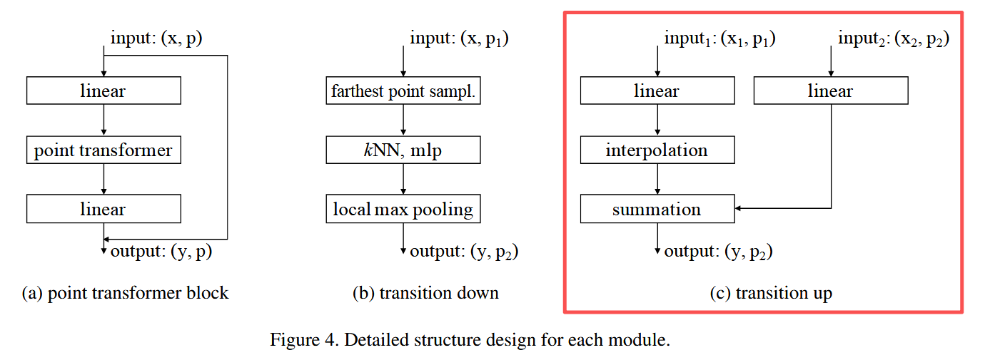
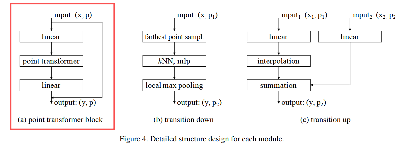
1.5 point Transformer block

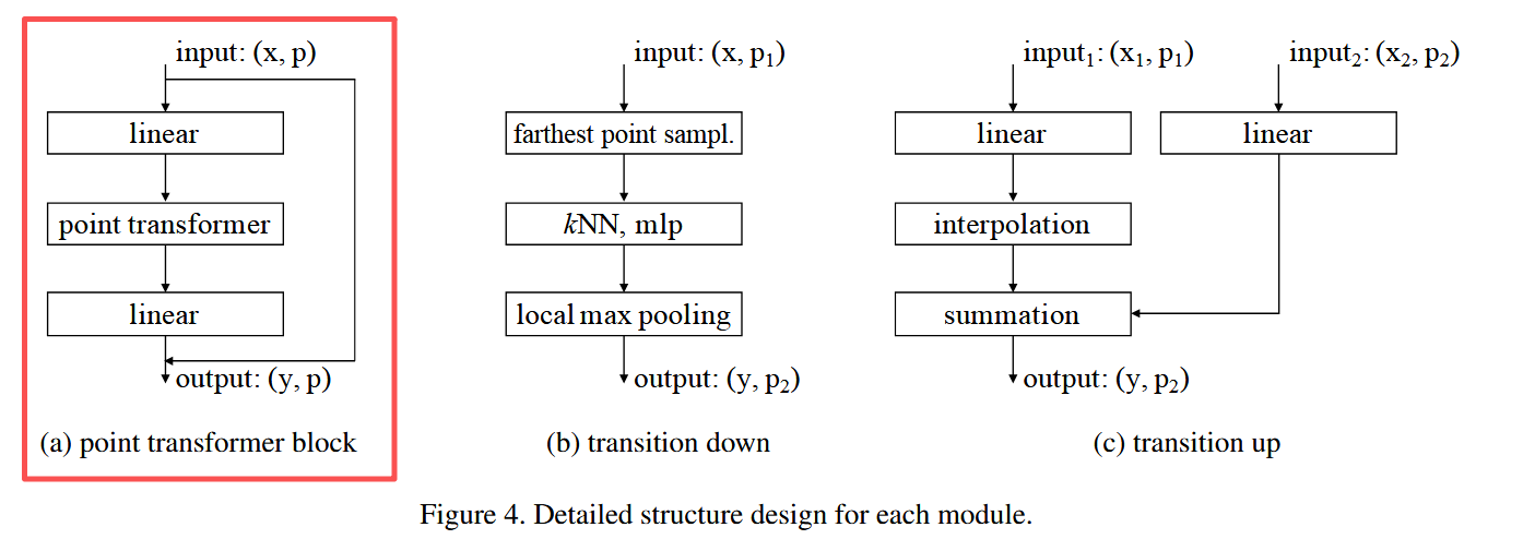
Point Transformer 模块是一个残差结构，如图 4(a) 所示。它包含：

• Point Transformer 层（核心）

• 降维的线性投影（加速计算）

• 残差连接

输入是一组点的特征向量及其 3D 坐标，输出是更新后的点特征。该模块在特征内容和三维空间布局上都能自适应进行信息聚合。

1.6 网络结构

整体的网络结构不复杂，分割的话类似 unet 型；分类的话就是串联。

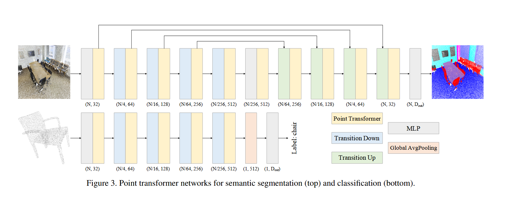
1.6.1 骨干网络

语义分割/分类的特征编码器有 5 个阶段，下采样率为 [1,4,4,4,4]，输出点数依次为 [N, N/4, N/16, N/64, N/256]。相邻阶段通过转换模块连接：

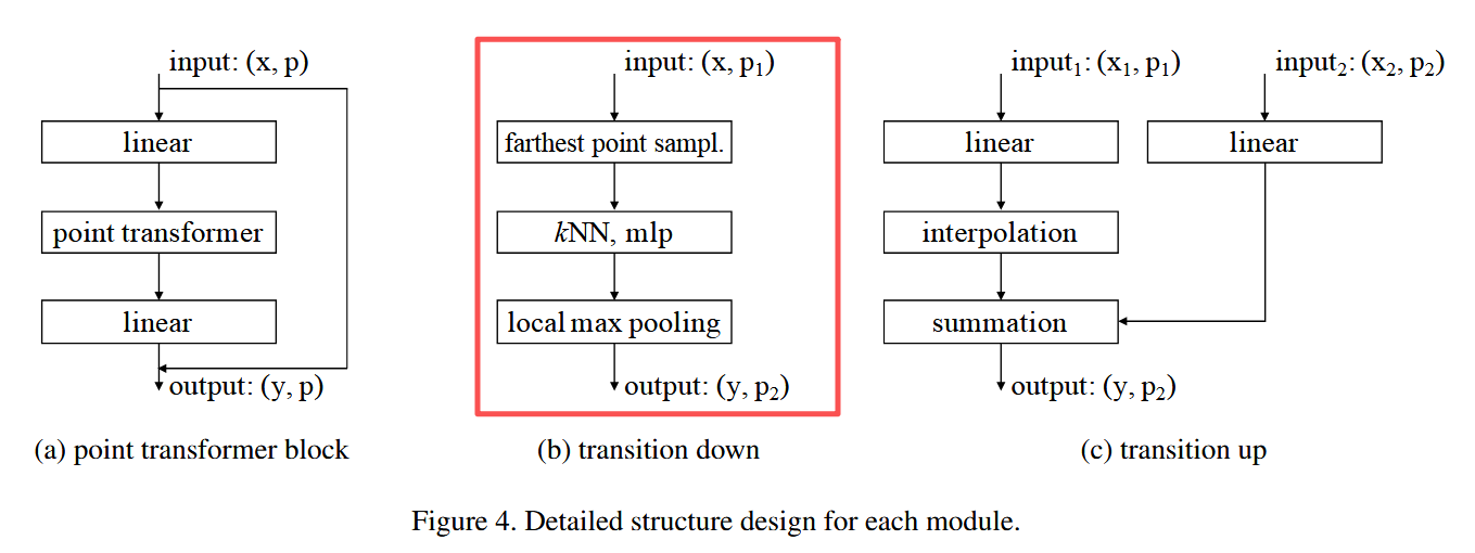
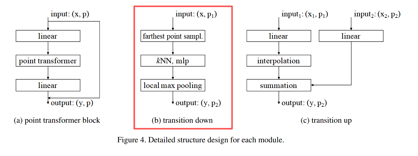
1.6.2 下采样

下采样过程如下图所示，

从 $P_1$ 采样子集 $P_2$（最远点采样），并将 $P_1$ 的特征汇聚到 $P_2$。流程：

• 线性层 → BN → ReLU
• kNN 聚合（k=16）
• max pooling

1.6.3 上采样

Transition up（图 4c）：

在解码阶段，将 $P_2$ 的特征映射回更高分辨率点集 $P_1$：

• 线性层 → BN → ReLU
• 三线性插值 *融合来自编码器的跳跃连接特征

1.6.4 分类/分割头

输出头：

语义分割：为每个点生成特征 → MLP → 每点分类 logits

分类任务：对点特征全局平均池化 → 全局特征向量 → MLP → 分类 logits

1.7 代码

1.7.1 Point Transformer Layer

1. 特征变换：将输入特征通过线性层生成 Q、K、V 三元组

2. 邻域构建：利用 KNN 算法为每个点构建局部邻域

3. 位置编码：将相对坐标通过 MLP 网络映射到高维特征空间

4. 注意力计算：结合特征差值和位置编码生成向量化注意力权重

5. 特征聚合：基于注意力权重对邻域特征进行加权融合

class PointTransformerLayer(nn.Module):def __init__(self, in_planes, out_planes, share_planes=8, nsample=16):super().__init__()# 中间通道数，简化处理（这里直接等于 out_planes）self.mid_planes = mid_planes = out_planes // 1self.out_planes = out_planesself.share_planes = share_planesself.nsample = nsample# Q, K, V 的线性变换self.linear_q = nn.Linear(in_planes, mid_planes)   # 查询向量 (query)self.linear_k = nn.Linear(in_planes, mid_planes)   # 键向量 (key)self.linear_v = nn.Linear(in_planes, out_planes)   # 值向量 (value)# 位置编码 δ (论文 Eq.(4): δ = θ(pi − pj))# 输入是相对坐标 (3D)，输出是与 out_planes 对齐的特征self.linear_p = nn.Sequential(nn.Linear(3, 3),nn.BatchNorm1d(3),nn.ReLU(inplace=True),nn.Linear(3, out_planes))# 权重生成函数 γ (MLP)，作用在 (q - k + δ) 上# 注意这里做了“通道分组”（share_planes），减少计算量self.linear_w = nn.Sequential(nn.BatchNorm1d(mid_planes),nn.ReLU(inplace=True),nn.Linear(mid_planes, mid_planes // share_planes),nn.BatchNorm1d(mid_planes // share_planes),nn.ReLU(inplace=True),nn.Linear(mid_planes // share_planes, out_planes // share_planes))# softmax 用来对注意力权重归一化self.softmax = nn.Softmax(dim=1)def forward(self, pxo) -> torch.Tensor:# 输入:# p: 点的坐标 (n, 3)# x: 点的特征 (n, c)# o: batch 索引 (b)p, x, o = pxo#  step1 得到 Q, K, Vx_q, x_k, x_v = self.linear_q(x), self.linear_k(x), self.linear_v(x)  # (n, c)# -------------------------------------------# step2 构建邻域 (kNN)，并返回局部邻域的特征# x_k: (n, nsample, 3+c)，包含相对坐标和 K 特征# x_v: (n, nsample, c)，邻域内的 V 特征x_k = pointops.queryandgroup(self.nsample, p, p, x_k, None, o, o, use_xyz=True) # (n, nsample, 3+c)x_v = pointops.queryandgroup(self.nsample, p, p, x_v, None, o, o, use_xyz=False) # (n, nsample, c)# -------------------------------------------# step3 分离相对坐标 p_r 和邻域内的 K 特征# p_r: (n, nsample, 3), x_k: (n, nsample, c)p_r, x_k = x_k[:, :, 0:3], x_k[:, :, 3:]# 将相对坐标 p_r 输入位置编码 MLP θ# 这里因为 BatchNorm 的维度问题，需要转置 (n, nsample, 3) ↔ (n, 3, nsample)for i, layer in enumerate(self.linear_p):p_r = layer(p_r.transpose(1, 2).contiguous()).transpose(1, 2).contiguous() \if i == 1 else layer(p_r)# 经过 MLP 后: (n, nsample, out_planes)# -------------------------------------------# step4 根据 Eq.(3): w = γ(φ(xi) − ψ(xj) + δ)# x_q.unsqueeze(1): (n, 1, c)，与邻域对齐# p_r reshape 后与 x_k 对齐做相加w = x_k - x_q.unsqueeze(1) + p_r.view(p_r.shape[0], p_r.shape[1], self.out_planes // self.mid_planes, self.mid_planes).sum(2)  # (n, nsample, c)# 将 w 输入 γ MLP (linear_w)，得到注意力权重for i, layer in enumerate(self.linear_w):w = layer(w.transpose(1, 2).contiguous()).transpose(1, 2).contiguous() if i % 3 == 0 else layer(w)# softmax 归一化注意力权重w = self.softmax(w)  # (n, nsample, c)# -------------------------------------------# step5 最终聚合 (Eq.(3) 中 ρ(...)*α(xj+δ))n, nsample, c = x_v.shapes = self.share_planesx = ((x_v + p_r).view(n, nsample, s, c // s) * w.unsqueeze(2)).sum(1).view(n, c)return x

稍微解释以下：
输入的是 pxo,可以分解

# p: 点的坐标 (n, 3)
# x: 点的特征 (n, c)
# o: batch 索引 (b)
p, x, o = pxo

p 一组点，x 是这组点对应的特征，o 是这组点对应的 batch 索引，也就是这组点属于哪个 batch

对这组特征 x 进行映射

#  step1 得到 Q, K, V
x_q, x_k, x_v = self.linear_q(x), self.linear_k(x), self.linear_v(x)  # (n, c)

构建 KNN,看最后的返回值，可以是特征，也是可以坐标+特征。所以：

# x_k: (n, nsample, 3+c)，包含相对坐标和 K 特征
# x_v: (n, nsample, c)，邻域内的 V 特征

这里 p_r 是相对坐标，具体可以看面代码“# >>>>>>>相对坐标<<<<<<”这里。

# step3 分离相对坐标 p_r 和邻域内的 K 特征
# p_r: (n, nsample, 3), x_k: (n, nsample, c)
p_r, x_k = x_k[:, :, 0:3], x_k[:, :, 3:]

这里的领域 查询主要是以下：

1. 邻域查询：对于查询点集合中的每个点，利用 KNN 算法在所有点集合中寻找最近的 nsample 个邻居点，并返回这些邻居点的索引；

2. 相对坐标计算：将每个查询点的邻居点坐标减去查询点自身坐标，得到以查询点为原点的局部相对坐标系；

3. 特征分组：根据邻居点索引，提取对应的特征向量，形成每个查询点的邻域特征集合。

该方法的核心作用是将无序的点云数据转换为有序的局部邻域结构，为后续的注意力计算提供空间上下文信息。

def queryandgroup(nsample, xyz, new_xyz, feat, idx, offset, new_offset, use_xyz=True):"""input: xyz: (n, 3), new_xyz: (m, 3), feat: (n, c), idx: (m, nsample), offset: (b), new_offset: (b)output: new_feat: (m, c+3, nsample), grouped_idx: (m, nsample)"""assert xyz.is_contiguous() and new_xyz.is_contiguous() and feat.is_contiguous()if new_xyz is None:new_xyz = xyzif idx is None:idx, _ = knnquery(nsample, xyz, new_xyz, offset, new_offset) # (m, nsample)n, m, c = xyz.shape[0], new_xyz.shape[0], feat.shape[1]grouped_xyz = xyz[idx.view(-1).long(), :].view(m, nsample, 3) # (m, nsample, 3)#grouped_xyz = grouping(xyz, idx) # (m, nsample, 3)grouped_xyz -= new_xyz.unsqueeze(1) # (m, nsample, 3) # >>>>>>>相对坐标<<<<<<grouped_feat = feat[idx.view(-1).long(), :].view(m, nsample, c) # (m, nsample, c)#grouped_feat = grouping(feat, idx) # (m, nsample, c)if use_xyz:return torch.cat((grouped_xyz, grouped_feat), -1) # (m, nsample, 3+c)else:return grouped_feat

计算注意力权重: 领域内最近邻键特征 - 领域所在中心点查询特征 + 相对位置编码

x_k 是领域特征，x_q 是中心点特征，p_r 是相对位置编码

# step4 根据 Eq.(3): w = γ(φ(xi) − ψ(xj) + δ)
# x_q.unsqueeze(1): (n, 1, c)，与邻域对齐
# p_r reshape 后与 x_k 对齐做相加
w = x_k - x_q.unsqueeze(1) + p_r.view(p_r.shape[0], p_r.shape[1], self.out_planes // self.mid_planes, self.mid_planes
).sum(2)  # (n, nsample, c)

最后，

# step5 最终聚合 (Eq.(3) 中 ρ(...)*α(xj+δ))
n, nsample, c = x_v.shape
s = self.share_planes
x = ((x_v + p_r).view(n, nsample, s, c // s) * w.unsqueeze(2)).sum(1).view(n, c)

w 对应下图的 bb，前面的对应 aa。

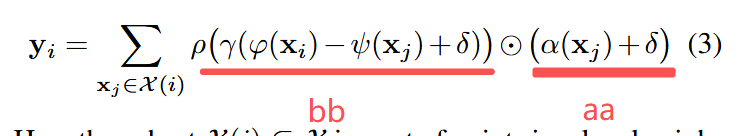
聚合: 对每个中心点的所有邻居点的特征在特征维度上进行分组，做通道分组(类似多头注意力，但是作用不完全相同) + 利用广播后做逐元素相乘，完成对同一个邻居点的所有通道分组应用相同权重分配的过程 + 所有邻居点特征进行求和，完成领域值信息聚合过程 + 多头重组回原貌

# （200，8，8，4） * （200，8，1，4） -> (200, 8, 8, 4) -> (200,8,4) -> (200,32)
x = ((x_v + p_r).view(n, nsample, s, c // s) * w.unsqueeze(2)).sum(1).view(n, c)

1.7.2 Transformer Block

主要是有一个残差连接

class PointTransformerBlock(nn.Module):"""Point Transformer 残差块实现预激活（Pre-Activation）的残差连接结构"""expansion = 1  # 维度扩展系数，1表示输出维度与输入维度相同def __init__(self, in_planes, planes, share_planes=8, nsample=16):"""初始化函数Args:in_planes: 输入特征维度planes: 中间特征维度（也是输出维度，因为expansion=1）share_planes: 通道分组数，用于减少计算量nsample: 每个点的邻居数量，用于kNN搜索"""super(PointTransformerBlock, self).__init__()# 第一层：线性变换 + 批归一化（升维或保持维度）self.linear1 = nn.Linear(in_planes, planes, bias=False)  # 无偏置，因为后面有BNself.bn1 = nn.BatchNorm1d(planes)  # 批归一化，加速训练# 核心：Point Transformer 自注意力层self.transformer2 = PointTransformerLayer(planes, planes, share_planes, nsample)self.bn2 = nn.BatchNorm1d(planes)  # Transformer后的批归一化# 第三层：线性变换 + 批归一化（调整到最终输出维度）self.linear3 = nn.Linear(planes, planes * self.expansion, bias=False)self.bn3 = nn.BatchNorm1d(planes * self.expansion)  # 最终批归一化# 激活函数（原地操作节省内存）self.relu = nn.ReLU(inplace=True)# 注意：这里应该有残差连接的shortcut处理# 如果 in_planes != planes * expansion，需要投影层if in_planes != planes * self.expansion:self.shortcut = nn.Sequential(nn.Linear(in_planes, planes * self.expansion, bias=False),nn.BatchNorm1d(planes * self.expansion))else:self.shortcut = nn.Identity()  # 恒等映射def forward(self, pxo):"""前向传播Args:pxo: 元组 (p, x, o)p: 点坐标，形状 (n, 3)x: 点特征，形状 (n, in_planes)o: 批次索引，形状 (b)Returns:元组 (p, x, o): 变换后的点坐标、特征和批次索引"""p, x, o = pxo  # 解包：点坐标, 点特征, batch索引# 保存原始输入用于残差连接（需要处理维度匹配）identity = x# 第一层：线性变换 → BN → ReLUx = self.linear1(x)      # (n, in_planes) → (n, planes)x = self.bn1(x)          # 批归一化x = self.relu(x)         # ReLU激活# 第二层：Point Transformer 自注意力 → BN → ReLUx = self.transformer2([p, x, o])  # 应用自注意力，形状 (n, planes)x = self.bn2(x)          # 批归一化x = self.relu(x)         # ReLU激活# 第三层：线性变换 → BNx = self.linear3(x)      # (n, planes) → (n, planes * expansion)x = self.bn3(x)          # 最终批归一化# 残差连接：处理维度匹配问题identity = self.shortcut(identity)  # 如果需要，投影到相同维度# 残差连接 + 激活x += identity            # 添加残差连接x = self.relu(x)         # 最终ReLU激活# 返回相同格式的数据return [p, x, o]

1.7.3 下采样

这部分主要有：

1. 最远点采样，
2. KNN 查询，
3. mlp,pool

其中最远点采样：

1. 初始化：随机选择一个起始点

2. 迭代选择：

   • 计算所有点到已选点集的最小距离
   • 选择距离最大的点（即最远的点）
   • 重复直到选择足够多的点

class TransitionDown(nn.Module):"""点云下采样过渡层功能：降低点云分辨率同时增加特征维度，保持批处理信息"""def __init__(self, in_planes, out_planes, stride=1, nsample=16):"""初始化下采样层Args:in_planes: 输入特征维度out_planes: 输出特征维度stride: 下采样步长（stride=1表示无下采样，只做特征变换）nsample: 邻域采样点数，用于局部特征聚合"""super().__init__()self.stride = stride    # 下采样率self.nsample = nsample  # 邻域采样数if stride != 1:# 下采样模式：需要处理坐标和特征，输出维度为3+in_planesself.linear = nn.Linear(3 + in_planes, out_planes, bias=False)  # 无偏置，因为后面有BNself.pool = nn.MaxPool1d(nsample)  # 最大池化，聚合邻域特征else:# 无下采样模式：只做特征变换self.linear = nn.Linear(in_planes, out_planes, bias=False)# 共享的批归一化和激活函数self.bn = nn.BatchNorm1d(out_planes)  # 批归一化self.relu = nn.ReLU(inplace=True)     # ReLU激活函数（原地操作节省内存）def forward(self, pxo):"""前向传播Args:pxo: 元组 (p, x, o)p: 点坐标，形状 (n, 3)x: 点特征，形状 (n, in_planes)o: 批次索引，形状 (b) - 每个元素表示该批次点的结束索引Returns:元组 (p, x, o): 下采样后的点坐标、特征和批次索引"""p, x, o = pxo  # 解包：点坐标, 点特征, 批次索引if self.stride != 1:# ==================== 下采样模式 ====================# 计算下采样后的批次索引 n_on_o, count = [o[0].item() // self.stride], o[0].item() // self.stridefor i in range(1, o.shape[0]):# 计算每个批次下采样后的点数count += (o[i].item() - o[i-1].item()) // self.striden_o.append(count)n_o = torch.IntTensor(n_o).to(o.device)  # 转换为张量并保持设备一致# 1. 最远点采样：从原始点云中选择代表性点idx = pointops.furthestsampling(p, o, n_o)  # (m) - 采样点索引，m为下采样后的点数n_p = p[idx.long(), :]  # (m, 3) - 下采样后的点坐标# 2. 查询和分组：为每个采样点找到邻域并聚合特征# 输出形状: (m, 3 + in_planes, nsample)# 包含：相对坐标(3) + 原始特征(in_planes)x = pointops.queryandgroup(self.nsample, p, n_p, x, None, o, n_o, use_xyz=True)# 3. 线性变换 + BN + ReLU# 先将特征维度转到最后： (m, 3+c, nsample) → (m, nsample, 3+c)x = self.linear(x.transpose(1, 2).contiguous())  # (m, nsample, out_planes)x = self.bn(x.transpose(1, 2).contiguous())      # (m, out_planes, nsample) - BN要求通道维度在前x = self.relu(x)                                # ReLU激活# 4. 最大池化：在邻域维度上池化，得到每个点的最终特征x = self.pool(x)          # (m, out_planes, 1) - 沿nsample维度池化x = x.squeeze(-1)         # (m, out_planes) - 移除最后一个维度# 更新点和批次信息p, o = n_p, n_o  # 使用下采样后的点坐标和批次索引else:# ==================== 无下采样模式 ====================# 只进行特征变换：Linear → BN → ReLUx = self.linear(x)    # (n, in_planes) → (n, out_planes)x = self.bn(x)        # 批归一化x = self.relu(x)      # ReLU激活# 返回相同格式的数据return [p, x, o]

1.7.4 上采样

class TransitionUp(nn.Module):"""点云上采样过渡层功能：恢复点云分辨率并融合不同层级的特征，实现特征上采样类似于CNN中的上采样/转置卷积层，但专为点云设计"""def __init__(self, in_planes, out_planes=None):"""初始化上采样层Args:in_planes: 输入特征维度out_planes: 输出特征维度（如果为None，则输出维度与输入相同）"""super().__init__()if out_planes is None:# 模式1：输出维度与输入相同（通常用于解码器中间层）self.linear1 = nn.Sequential(nn.Linear(2 * in_planes, in_planes),  # 将拼接后的特征映射回原维度nn.BatchNorm1d(in_planes),            # 批归一化nn.ReLU(inplace=True)                 # ReLU激活)self.linear2 = nn.Sequential(nn.Linear(in_planes, in_planes),      # 全局特征变换nn.ReLU(inplace=True)                 # ReLU激活)else:# 模式2：改变输出维度（通常用于连接编码器和解码器）self.linear1 = nn.Sequential(nn.Linear(out_planes, out_planes),    # 恒等映射变换nn.BatchNorm1d(out_planes),           # 批归一化nn.ReLU(inplace=True)                 # ReLU激活)self.linear2 = nn.Sequential(nn.Linear(in_planes, out_planes),     # 维度变换nn.BatchNorm1d(out_planes),           # 批归一化nn.ReLU(inplace=True)                 # ReLU激活)def forward(self, pxo1, pxo2=None):"""前向传播：两种模式Mode 1 (pxo2 is None): 仅使用全局特征增强当前层特征Mode 2 (pxo2 provided): 跳跃连接 - 融合深层特征和浅层特征Args:pxo1: 元组 (p, x, o) - 当前层的点坐标、特征、批次索引pxo2: 元组 (p, x, o) - 跳跃连接来自编码器的点坐标、特征、批次索引（可选）Returns:x: 上采样后的特征，形状与pxo1中的特征相同或变换后的维度"""if pxo2 is None:# ==================== 模式1：全局特征增强 ====================# 仅使用当前层特征进行自增强（无跳跃连接）_, x, o = pxo1  # 解包：忽略坐标，只取特征和批次索引x_tmp = []  # 存储处理后的每个批次特征# 按批次处理for i in range(o.shape[0]):# 计算当前批次的起始、结束索引和点数if i == 0:s_i, e_i, cnt = 0, o[0].item(), o[0].item()  # 第一个批次else:s_i, e_i = o[i-1].item(), o[i].item()        # 后续批次cnt = e_i - s_i                              # 当前批次点数# 提取当前批次的特征x_b = x[s_i:e_i, :]  # (cnt, in_planes)# 计算全局平均特征并变换global_feat = x_b.sum(0, keepdim=True) / cnt  # (1, in_planes) - 批次平均特征transformed_global = self.linear2(global_feat)  # (1, in_planes) - 变换后的全局特征# 将全局特征复制到每个点，并与原始特征拼接x_b = torch.cat((x_b, transformed_global.repeat(cnt, 1)), dim=1)  # (cnt, 2*in_planes)x_tmp.append(x_b)# 合并所有批次x = torch.cat(x_tmp, 0)  # (n, 2*in_planes)# 最终变换：降维 + 激活x = self.linear1(x)  # (n, in_planes)else:# ==================== 模式2：跳跃连接特征融合 ====================# 融合编码器（深层）和解码器（浅层）的特征p1, x1, o1 = pxo1  # 当前层（解码器）：通常分辨率更高p2, x2, o2 = pxo2  # 跳跃连接层（编码器）：通常特征更抽象# 处理当前层特征x1_transformed = self.linear1(x1)  # (n1, out_planes)# 处理跳跃连接特征并进行上采样（插值）x2_transformed = self.linear2(x2)  # (n2, out_planes)# 将深层特征上采样到浅层分辨率：通过点云插值# 将p2位置的特征插值到p1位置x2_upsampled = pointops.interpolation(p2, p1, x2_transformed, o2, o1)# 特征融合：当前层特征 + 上采样的编码器特征x = x1_transformed + x2_upsampled  # 逐元素相加return x

该插值流程就是： 对每个目标点，找到源点云的 k 个最近邻 → 根据反距离加权分配权重 → 用邻居特征加权求和 → 得到目标点特征。

def interpolation(xyz, new_xyz, feat, offset, new_offset, k=3):"""点云特征插值函数（基于 KNN + 反距离加权）Args:xyz: (m, 3) 源点云坐标（低分辨率点云，比如 encoder 输出）new_xyz: (n, 3) 目标点云坐标（高分辨率点云，比如 decoder 对应层）feat: (m, c) 源点云的特征offset: (b) 每个 batch 的点数累积和（源点云）new_offset: (b) 每个 batch 的点数累积和（目标点云）k: int，插值时选取的近邻点个数（默认3）Returns:new_feat: (n, c)，插值到目标点上的特征"""# 确保输入 tensor 在内存中是连续存放的，提高计算效率assert xyz.is_contiguous() and new_xyz.is_contiguous() and feat.is_contiguous()# 在源点云 xyz 中，查找目标点云 new_xyz 的 k 个最近邻# idx: (n, k) 最近邻点索引# dist: (n, k) 最近邻点对应的欧氏距离idx, dist = knnquery(k, xyz, new_xyz, offset, new_offset)  # (n, 3), (n, 3)# 计算距离的倒数，避免除零加一个小量dist_recip = 1.0 / (dist + 1e-8)  # (n, k)# 对权重进行归一化，使每个点的权重和为 1norm = torch.sum(dist_recip, dim=1, keepdim=True)  # (n, 1)weight = dist_recip / norm  # (n, k)# 初始化插值后的特征 (n, c)，全零new_feat = torch.zeros((new_xyz.shape[0], feat.shape[1]), dtype=feat.dtype)# 遍历每个近邻点（这里默认 k=3）for i in range(k):indices = idx[:, i].long()  # 第 i 个邻居的索引# 有效性检查：确保索引在合法范围内valid_mask = (indices >= 0) & (indices < feat.shape[0])if valid_mask.any():# 对有效邻居点：加权累加特征# feat[indices] : (n, c) 邻居点特征# weight[:, i].unsqueeze(-1) : (n, 1) 权重# → 逐点乘法，最后累加到 new_featnew_feat[valid_mask] += feat[indices[valid_mask], :] * weight[valid_mask, i].unsqueeze(-1)return new_feat

1.7.5 模型主体

class PointTransformerSeg(nn.Module):"""Point Transformer 用于点云语义分割的网络采用编码器-解码器结构（类似 U-Net），编码器用于下采样和提取抽象特征，解码器用于上采样和特征融合，最终输出每个点的类别概率。"""def __init__(self, block, blocks, c=6, k=13):"""Args:block: 点变换模块类型（Point Transformer Block）blocks: 每一层包含 block 数量列表c: 输入点特征维度（通常是 xyz + 额外特征）k: 分类类别数量"""super().__init__()self.c = cself.in_planes, planes = c, [32, 64, 128, 256, 512]  # 编码器各层输出通道fpn_planes, fpnhead_planes, share_planes = 128, 64, 8stride, nsample = [1, 4, 4, 4, 4], [8, 16, 16, 16, 16]  # 下采样比例与邻居点数# ========== 编码器 ==========# enc1: 分辨率 N/1self.enc1 = self._make_enc(block, planes[0], blocks[0], share_planes, stride=stride[0], nsample=nsample[0])# enc2: 分辨率 N/4self.enc2 = self._make_enc(block, planes[1], blocks[1], share_planes, stride=stride[1], nsample=nsample[1])# enc3: 分辨率 N/16self.enc3 = self._make_enc(block, planes[2], blocks[2], share_planes, stride=stride[2], nsample=nsample[2])# enc4: 分辨率 N/64self.enc4 = self._make_enc(block, planes[3], blocks[3], share_planes, stride=stride[3], nsample=nsample[3])# enc5: 分辨率 N/256self.enc5 = self._make_enc(block, planes[4], blocks[4], share_planes, stride=stride[4], nsample=nsample[4])# ========== 解码器 ==========# dec5: 解码器最深层，转换 p5 特征（is_head=True 表示输出头，不进行 skip 融合）self.dec5 = self._make_dec(block, planes[4], 2, share_planes, nsample=nsample[4], is_head=True)# dec4: 融合 p5 与 p4self.dec4 = self._make_dec(block, planes[3], 2, share_planes, nsample=nsample[3])# dec3: 融合 p4 与 p3self.dec3 = self._make_dec(block, planes[2], 2, share_planes, nsample=nsample[2])# dec2: 融合 p3 与 p2self.dec2 = self._make_dec(block, planes[1], 2, share_planes, nsample=nsample[1])# dec1: 融合 p2 与 p1self.dec1 = self._make_dec(block, planes[0], 2, share_planes, nsample=nsample[0])# 分类头：每个点输出 k 个类别得分self.cls = nn.Sequential(nn.Linear(planes[0], planes[0]),nn.BatchNorm1d(planes[0]),nn.ReLU(inplace=True),nn.Linear(planes[0], k))# ========== 构建编码器层 ==========def _make_enc(self, block, planes, blocks, share_planes=8, stride=1, nsample=16):layers = []# TransitionDown: 点云下采样 + 特征升维layers.append(TransitionDown(self.in_planes, planes * block.expansion, stride, nsample))self.in_planes = planes * block.expansion# 后续 block 叠加处理下采样后的特征for _ in range(1, blocks):layers.append(block(self.in_planes, self.in_planes, share_planes, nsample=nsample))return nn.Sequential(*layers)# ========== 构建解码器层 ==========def _make_dec(self, block, planes, blocks, share_planes=8, nsample=16, is_head=False):layers = []# TransitionUp: 点云上采样 + 特征融合# is_head=True 时表示输出层，不进行 skip 融合layers.append(TransitionUp(self.in_planes, None if is_head else planes * block.expansion))self.in_planes = planes * block.expansion# 后续 block 叠加处理上采样后的特征for _ in range(1, blocks):layers.append(block(self.in_planes, self.in_planes, share_planes, nsample=nsample))return nn.Sequential(*layers)# ========== 前向传播 ==========def forward(self, pxo):"""Args:pxo: tuple (p0, x0, o0)p0: (n,3) 点坐标x0: (n,c) 点特征o0: (b) 每个 batch 的点累积偏移Returns:x: (n,k) 每个点的类别预测"""p0, x0, o0 = pxo# 如果输入特征只有 xyz，直接使用 p0，否则拼接额外特征x0 = p0 if self.c == 3 else torch.cat((p0, x0), 1)# ================= 编码器 =================p1, x1, o1 = self.enc1([p0, x0, o0])p2, x2, o2 = self.enc2([p1, x1, o1])p3, x3, o3 = self.enc3([p2, x2, o2])p4, x4, o4 = self.enc4([p3, x3, o3])p5, x5, o5 = self.enc5([p4, x4, o4])# ================= 解码器 =================# 注意 decX[0] 是 TransitionUp，上采样层# decX[1:] 是 Point Transformer Block，处理上采样后的特征x5 = self.dec5[1:]([p5, self.dec5[0]([p5, x5, o5]), o5])[1]x4 = self.dec4[1:]([p4, self.dec4[0]([p4, x4, o4], [p5, x5, o5]), o4])[1]x3 = self.dec3[1:]([p3, self.dec3[0]([p3, x3, o3], [p4, x4, o4]), o3])[1]x2 = self.dec2[1:]([p2, self.dec2[0]([p2, x2, o2], [p3, x3, o3]), o2])[1]x1 = self.dec1[1:]([p1, self.dec1[0]([p1, x1, o1], [p2, x2, o2]), o1])[1]# ================= 分类头 =================x = self.cls(x1)  # 输出每个点的 k 类得分return x

参考

1. https://binaryoracle.github.io/3DVL/PointTransformer.html#%E5%BC%95%E8%A8%80
2. https://www.cnblogs.com/xiaxuexiaoab/p/18258314
3. https://github.heygears.com/POSTECH-CVLab/point-transformer?tab=readme-ov-file