线性代数 · SVD | 几何本质、求解方法与应用

注：英文引文，机翻未校。
如有内容异常，请看原文。

---

We Recommend a Singular Value Decomposition

奇异值分解推荐

Posted August 2009.

In this article, we will offer a geometric explanation of singular value decompositions and look at some of the applications of them.
本文将对奇异值分解进行几何解释，并探讨其一些应用。

David Austin
Grand Valley State University
david at merganser.math.gvsu.edu

Introduction

引言

The topic of this article, the singular value decomposition, is one that should be a part of the standard mathematics undergraduate curriculum but all too often slips between the cracks. Besides being rather intuitive, these decompositions are incredibly useful. For instance, Netflix, the online movie rental company, is currently offering a $$1$ million prize for anyone who can improve the accuracy of its movie recommendation system by $10\%$. Surprisingly, this seemingly modest problem turns out to be quite challenging, and the groups involved are now using rather sophisticated techniques. At the heart of all of them is the singular value decomposition.
本文的主题——奇异值分解——本应是数学本科课程的标准内容，但却常常被忽视。这种分解不仅相当直观，而且极其有用。例如，Netflix——一家在线电影租赁公司——目前正在悬赏 100 万美元，奖励任何能够将其电影推荐系统的准确性提高 10% 的人。令人惊讶的是，这个看似简单的问题实际上相当具有挑战性，而参与其中的团队现在正在使用相当复杂的技术。所有这些技术的核心都是奇异值分解。

A singular value decomposition provides a convenient way for breaking a matrix, which perhaps contains some data we are interested in, into simpler, meaningful pieces. In this article, we will offer a geometric explanation of singular value decompositions and look at some of the applications of them.
奇异值分解提供了一种方便的方法，可以将一个矩阵（其中可能包含我们感兴趣的数据）分解成更简单、更有意义的部分。在本文中，我们将对奇异值分解进行几何解释，并探讨其一些应用。

The geometry of linear transformations

线性变换的几何

Let us begin by looking at some simple matrices, namely those with two rows and two columns. Our first example is the diagonal matrix
让我们先来看一些简单的矩阵，即两行两列的矩阵。我们的第一个例子是对角矩阵

$$M=\left[\begin{array}{cc}3& 0\\ 0& 1\end{array}\right]$$

Geometrically, we may think of a matrix like this as taking a point $(\mathbf{x},\mathbf{y})$ in the plane and transforming it into another point using matrix multiplication:
从几何上讲，我们可以将这样的矩阵视为将平面上的一个点 $(\mathbf{x},\mathbf{y})$ 通过矩阵乘法变换为另一个点：

$$\left[\begin{array}{cc}3& 0\\ 0& 1\end{array}\right]\left[\begin{array}{c}x\\ y\end{array}\right]=\left[\begin{array}{c}3x\\ y\end{array}\right]$$

The effect of this transformation is shown below: the plane is horizontally stretched by a factor of $3$, while there is no vertical change.
这种变换的效果如下所示：平面在水平方向上被拉伸了 $3$ 倍，而垂直方向上没有变化。

Now let’s look at
现在我们来看

$$M=\left[\begin{array}{cc}2& 1\\ 1& 2\end{array}\right]$$

which produces this effect
它产生了如下效果

It is not so clear how to describe simply the geometric effect of the transformation. However, let’s rotate our grid through a $45$ degree angle and see what happens.
这种变换的几何效果并不容易简单描述。然而，让我们将网格旋转 $45$ 度，看看会发生什么。

Ah ha. We see now that this new grid is transformed in the same way that the original grid was transformed by the diagonal matrix: the grid is stretched by a factor of $3$ in one direction.
啊哈。我们现在看到，这个新的网格被变换的方式与原始网格被对角矩阵变换的方式相同：网格在一个方向上被拉伸了 $3$ 倍。

This is a very special situation that results from the fact that the matrix $M$ is symmetric; that is, the transpose of $M$, the matrix obtained by flipping the entries about the diagonal, is equal to $M$. If we have a symmetric $2\times 2$ matrix, it turns out that we may always rotate the grid in the domain so that the matrix acts by stretching and perhaps reflecting in the two directions. In other words, symmetric matrices behave like diagonal matrices.
这是一个非常特殊的情况，它是由矩阵 $M$ 是对称的这一事实导致的；也就是说，$M$ 的转置——通过对角线翻转条目得到的矩阵——等于 $M$。事实证明，如果我们有一个对称的 $2\times 2$ 矩阵，那么我们总是可以旋转定义域中的网格，使得矩阵通过在两个方向上拉伸和可能反射来起作用。换句话说，对称矩阵表现得像对角矩阵一样。

Said with more mathematical precision, given a symmetric matrix $M$, we may find a set of orthogonal vectors ${\mathbf{v}}_i$ so that $M{\mathbf{v}}_i$ is a scalar multiple of ${\mathbf{v}}_i$; that is
用更精确的数学语言来说，给定一个对称矩阵 $M$，我们可以找到一组正交向量 ${\mathbf{v}}_i$，使得 $M{\mathbf{v}}_i$ 是 ${\mathbf{v}}_i$ 的标量倍；也就是说

$$M{\mathbf{v}}_i={\lambda }_i{\mathbf{v}}_i$$

where ${\lambda }_i$ is a scalar. Geometrically, this means that the vectors ${\mathbf{v}}_i$ are simply stretched and/or reflected when multiplied by $M$. Because of this property, we call the vectors ${\mathbf{v}}_i$ eigenvectors of $M$; the scalars ${\lambda }_i$ are called eigenvalues. An important fact, which is easily verified, is that eigenvectors of a symmetric matrix corresponding to different eigenvalues are orthogonal.
其中 ${\lambda }_i$ 是一个标量。从几何上讲，这意味着当 ${\mathbf{v}}_i$ 乘以 $M$ 时，它们只是被拉伸和/或反射。由于这个性质，我们称向量 ${\mathbf{v}}_i$ 为 $M$ 的 特征向量；标量 ${\lambda }_i$ 称为 特征值。一个重要的事实（很容易验证）是，对应于不同特征值的对称矩阵的特征向量是正交的。

If we use the eigenvectors of a symmetric matrix to align the grid, the matrix stretches and reflects the grid in the same way that it does the eigenvectors.
如果我们使用对称矩阵的特征向量来对齐网格，那么矩阵会像对特征向量一样拉伸和反射网格。

The geometric description we gave for this linear transformation is a simple one: the grid is simply stretched in one direction. For more general matrices, we will ask if we can find an orthogonal grid that is transformed into another orthogonal grid. Let’s consider a final example using a matrix that is not symmetric:
我们对这个线性变换的几何描述很简单：网格只是在一个方向上被拉伸。对于更一般的矩阵，我们会问：是否可以找到一个正交网格，使其被变换为另一个正交网格？让我们考虑最后一个例子，使用一个非对称矩阵：

$$M=\left[\begin{array}{cc}1& 1\\ 0& 1\end{array}\right]$$

This matrix produces the geometric effect known as a shear.
这个矩阵产生了被称为 剪切 的几何效果。

It’s easy to find one family of eigenvectors along the horizontal axis. However, our figure above shows that these eigenvectors cannot be used to create an orthogonal grid that is transformed into another orthogonal grid. Nonetheless, let’s see what happens when we rotate the grid first by $30$ degrees,
很容易在水平轴上找到一族特征向量。然而，上面的图形显示，这些特征向量不能用来创建一个被变换为另一个正交网格的正交网格。尽管如此，让我们看看当我们首先将网格旋转 $30$ 度时会发生什么：

Notice that the angle at the origin formed by the red parallelogram on the right has increased. Let’s next rotate the grid by $60$ degrees.
注意，右边的红色平行四边形在原点处形成的角度增加了。接下来，让我们将网格旋转 $60$ 度。

Hmm. It appears that the grid on the right is now almost orthogonal. In fact, by rotating the grid in the domain by an angle of roughly $58.28$ degrees, both grids are now orthogonal.
嗯。看起来右边的网格现在几乎是正交的。事实上，通过将定义域中的网格旋转大约 $58.28$ 度，两个网格现在都是正交的。

The singular value decomposition

奇异值分解

This is the geometric essence of the singular value decomposition for $2\times 2$ matrices: for any $2\times 2$ matrix, we may find an orthogonal grid that is transformed into another orthogonal grid.
这就是 $2\times 2$ 矩阵奇异值分解的几何本质：对于任何 $2\times 2$ 矩阵，我们都可以找到一个被变换为另一个正交网格的正交网格。

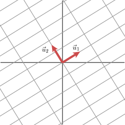
We will express this fact using vectors: with an appropriate choice of orthogonal unit vectors ${\mathbf{v}}_1$ and ${\mathbf{v}}_2$, the vectors $M{\mathbf{v}}_1$ and $M{\mathbf{v}}_2$ are orthogonal.
我们将用向量来表达这一事实：通过适当选择正交单位向量 ${\mathbf{v}}_1$ 和 ${\mathbf{v}}_2$，向量 $M{\mathbf{v}}_1$ 和 $M{\mathbf{v}}_2$ 是正交的。

We will use ${\mathbf{u}}_1$ and ${\mathbf{u}}_2$ to denote unit vectors in the direction of $M{\mathbf{v}}_1$ and $M{\mathbf{v}}_2$. The lengths of $M{\mathbf{v}}_1$ and $M{\mathbf{v}}_2$–denoted by ${\sigma }_1$ and ${\sigma }_2$–describe the amount that the grid is stretched in those particular directions. These numbers are called the singular values of $M$. (In this case, the singular values are the golden ratio and its reciprocal, but that is not so important here.)
我们将用 ${\mathbf{u}}_1$ 和 ${\mathbf{u}}_2$ 来表示 $M{\mathbf{v}}_1$ 和 $M{\mathbf{v}}_2$ 方向上的单位向量。$M{\mathbf{v}}_1$ 和 $M{\mathbf{v}}_2$ 的长度（用 ${\sigma }_1$ 和 ${\sigma }_2$ 表示）描述了网格在这些特定方向上被拉伸的程度。这些数字被称为 $M$ 的 奇异值。（在这种情况下，奇异值是黄金比例及其倒数，但这在这里并不重要。）

$$\left[\begin{array}{cc}{u}_1& u_2\end{array}\right]\left[\begin{array}{cc}{\sigma }_1& 0\\ 0& {\sigma }_2\end{array}\right]\left[\begin{array}{c}{v}_1^T\\ v_2^T\end{array}\right]$$

We therefore have
因此，我们有

$$\begin{gathered} M{\mathbf{v}}_1={\sigma }_1{\mathbf{u}}_1 \\ M{\mathbf{v}}_2={\sigma }_2{\mathbf{u}}_2 \end{gathered}$$

We may now give a simple description for how the matrix $M$ treats a general vector $\mathbf{x}$. Since the vectors ${\mathbf{v}}_1$ and ${\mathbf{v}}_2$ are orthogonal unit vectors, we have
现在我们可以简单描述矩阵 $M$ 如何处理一个一般的向量 $\mathbf{x}$。由于向量 ${\mathbf{v}}_1$ 和 ${\mathbf{v}}_2$ 是正交单位向量，我们有

$$\mathbf{x}=({\mathbf{v}}_1\cdot \mathbf{x}){\mathbf{v}}_1+({\mathbf{v}}_2\cdot \mathbf{x}){\mathbf{v}}_2$$

This means that
这意味着

$$\begin{gathered} M\mathbf{x}=({\mathbf{v}}_1\cdot \mathbf{x})M{\mathbf{v}}_1+({\mathbf{v}}_2\cdot \mathbf{x})M{\mathbf{v}}_2 \\ M\mathbf{x}=({\mathbf{v}}_1\cdot \mathbf{x}){\sigma }_1{\mathbf{u}}_1+({\mathbf{v}}_2\cdot \mathbf{x}){\sigma }_2{\mathbf{u}}_2 \end{gathered}$$

Remember that the dot product may be computed using the vector transpose
记住，点积可以用向量转置来计算

$$\mathbf{v}\cdot \mathbf{x}={\mathbf{v}}^T\mathbf{x}$$

which leads to
这导致

$$\begin{array}{rl}M\mathbf{x}& ={\mathbf{u}}_1{\sigma }_1{\mathbf{v}}_1^T\mathbf{x}+{\mathbf{u}}_2{\sigma }_2{\mathbf{v}}_2^T\mathbf{x}\\ M& ={\mathbf{u}}_1{\sigma }_1{\mathbf{v}}_1^T+{\mathbf{u}}_2{\sigma }_2{\mathbf{v}}_2^T\end{array}$$

This is usually expressed by writing
这通常写作

$$M=U\Sigma V^T$$

where $U$ is a matrix whose columns are the vectors ${\mathbf{u}}_1$ and ${\mathbf{u}}_2$, $\Sigma$ is a diagonal matrix whose entries are ${\sigma }_1$ and ${\sigma }_2$, and $V$ is a matrix whose columns are ${\mathbf{v}}_1$ and ${\mathbf{v}}_2$. The superscript $T$ on the matrix $V$ denotes the matrix transpose of $V$.
其中，$U$ 是一个矩阵，其列向量为 ${\mathbf{u}}_1$ 和 ${\mathbf{u}}_2$；$\Sigma$ 是一个对角矩阵，其条目为 ${\sigma }_1$ 和 ${\sigma }_2$；$V$ 是一个矩阵，其列向量为 ${\mathbf{v}}_1$ 和 ${\mathbf{v}}_2$。矩阵 $V$ 上的上标 $T$ 表示 $V$ 的矩阵转置。

This shows how to decompose the matrix $M$ into the product of three matrices: $V$ describes an orthonormal basis in the domain, and $U$ describes an orthonormal basis in the co-domain, and $\Sigma$ describes how much the vectors in $V$ are stretched to give the vectors in $U$.
这展示了如何将矩阵 $M$ 分解为三个矩阵的乘积：$V$ 描述定义域中的一个正交归一基，$U$ 描述值域中的一个正交归一基，$\Sigma$ 描述 $V$ 中的向量被拉伸多少以得到 $U$ 中的向量。

How do we find the singular decomposition?

如何找到奇异分解？

The power of the singular value decomposition lies in the fact that we may find it for any matrix. How do we do it?
奇异值分解的优势在于，我们可以为任意矩阵找到奇异值分解。具体该如何操作呢？

Let’s look at our earlier example and add the unit circle in the domain. Its image will be an ellipse whose major and minor axes define the orthogonal grid in the co-domain.
让我们回顾前面的例子，并在定义域中添加单位圆。单位圆经过矩阵变换后的图像是一个椭圆，该椭圆的长轴和短轴定义了值域中的正交网格。

Notice that the major and minor axes are defined by $M{\mathbf{v}}_1$ and $M{\mathbf{v}}_2$. These vectors therefore are the longest and shortest vectors among all the images of vectors on the unit circle.
注意，椭圆的长轴和短轴由 $M{\mathbf{v}}_1$ 和 $M{\mathbf{v}}_2$ 定义。因此，在单位圆上所有向量经过矩阵变换后的图像中，这两个向量分别是最长和最短的向量。

In other words, the function $|M\mathbf{x}|$ on the unit circle has a maximum at ${\mathbf{v}}_1$ and a minimum at ${\mathbf{v}}_2$. This reduces the problem to a rather standard calculus problem in which we wish to optimize a function over the unit circle. It turns out that the critical points of this function occur at the eigenvectors of the matrix $M^{T}M$. Since this matrix is symmetric, eigenvectors corresponding to different eigenvalues will be orthogonal. This gives the family of vectors ${\mathbf{v}}_i$.
换句话说，单位圆上的函数 $|M\mathbf{x}|$ 在 ${\mathbf{v}}_1$ 处取得最大值，在 ${\mathbf{v}}_2$ 处取得最小值。这将问题简化为一个标准的微积分优化问题——在单位圆上寻找函数的极值。研究表明，该函数的临界点恰好是矩阵 $M^{T}M$ 的特征向量。由于 $M^{T}M$ 是对称矩阵，对应于不同特征值的特征向量相互正交，由此我们得到了向量族 ${\mathbf{v}}_i$。

The singular values are then given by ${\sigma }_i=|M{\mathbf{v}}_i|$, and the vectors ${\mathbf{u}}_i$ are obtained as unit vectors in the direction of $M{\mathbf{v}}_i$. But why are the vectors ${\mathbf{u}}_i$ orthogonal?
奇异值由 ${\sigma }_i=|M{\mathbf{v}}_i|$ 定义，而向量 ${\mathbf{u}}_i$ 是 $M{\mathbf{v}}_i$ 方向上的单位向量。但为什么 ${\mathbf{u}}_i$ 是正交的呢？

To explain this, we will assume that ${\sigma }_i$ and ${\sigma }_j$ are distinct singular values. We have
为了说明这一点，我们假设 ${\sigma }_i$ 和 ${\sigma }_j$ 是不同的奇异值，且满足：

$$\begin{gathered} M{\mathbf{v}}_i={\sigma }_i{\mathbf{u}}_i \\ M{\mathbf{v}}_j={\sigma }_j{\mathbf{u}}_j \end{gathered}$$

Let’s begin by looking at the expression $M{\mathbf{v}}_i\cdot M{\mathbf{v}}_j$ and assuming, for convenience, that the singular values are non-zero. On one hand, this expression is zero since the vectors ${\mathbf{v}}_i$, which are eigenvectors of the symmetric matrix $M^{T}M$, are orthogonal to one another:
首先观察表达式 $M{\mathbf{v}}_i\cdot M{\mathbf{v}}_j$，为方便计算，假设奇异值非零。一方面，由于 ${\mathbf{v}}_i$ 是对称矩阵 $M^{T}M$ 的特征向量，且不同特征值对应的特征向量正交，因此该表达式的值为 0：

$$M{\mathbf{v}}_i\cdot M{\mathbf{v}}_j={\mathbf{v}}_i^T{M}^{T}M{\mathbf{v}}_j={\mathbf{v}}_i\cdot M^{T}M{\mathbf{v}}_j={\lambda }_j{\mathbf{v}}_i\cdot {\mathbf{v}}_j=0$$

$$\begin{array}{rl}M{\mathbf{v}}_i\cdot M{\mathbf{v}}_j& ={\mathbf{v}}_i^T(M^{T}M{\mathbf{v}}_j)\text{（内积与矩阵转置的等价性：}\mathbf{a}\cdot \mathbf{b}={\mathbf{a}}^T\mathbf{b}\text{）}\\ & ={\mathbf{v}}_i^T({\lambda }_j{\mathbf{v}}_j)\text{（因}{\mathbf{v}}_j\text{是}{M}^{T}M\text{的特征向量，故}{M}^{T}M{\mathbf{v}}_j={\lambda }_j{\mathbf{v}}_j\text{）}\\ & ={\lambda }_j({\mathbf{v}}_i^T{\mathbf{v}}_j)\text{（标量}{\lambda }_j\text{可提取到乘积外）}\\ & ={\lambda }_j({\mathbf{v}}_i\cdot {\mathbf{v}}_j)\text{（矩阵转置与内积的等价性：}{\mathbf{a}}^T\mathbf{b}=\mathbf{a}\cdot \mathbf{b}\text{）}\\ & ={\lambda }_j\cdot 0\text{（对称矩阵不同特征值对应的特征向量正交：}{\mathbf{v}}_i\cdot {\mathbf{v}}_j=0\text{）}\\ & =0\end{array}$$

On the other hand, we have
另一方面，我们可以将表达式展开为：

$$M{\mathbf{v}}_i\cdot M{\mathbf{v}}_j={\sigma }_i{\sigma }_j{\mathbf{u}}_i\cdot {\mathbf{u}}_j=0$$

Since ${\sigma }_i$ and ${\sigma }_j$ are non-zero, this implies ${\mathbf{u}}_i\cdot {\mathbf{u}}_j=0$. Therefore, ${\mathbf{u}}_i$ and ${\mathbf{u}}_j$ are orthogonal—we have found an orthogonal set of vectors ${\mathbf{v}}_i$ that is transformed into another orthogonal set ${\mathbf{u}}_i$. The singular values describe the amount of stretching in the different directions.
由于 ${\sigma }_i$ 和 ${\sigma }_j$ 非零，由此可推出 ${\mathbf{u}}_i\cdot {\mathbf{u}}_j=0$，即 ${\mathbf{u}}_i$ 和 ${\mathbf{u}}_j$ 正交。至此，我们找到了一组正交向量 ${\mathbf{v}}_i$，它们经过矩阵 $M$ 变换后仍为正交向量 ${\mathbf{u}}_i$，而奇异值则描述了不同方向上的拉伸程度。

In practice, this is not the procedure used to find the singular value decomposition of a matrix since it is not particularly efficient or well-behaved numerically.
在实际应用中，我们并不会采用上述方法计算奇异值分解——因为该方法在数值计算中效率较低，且稳定性较差。

Another example

另一个例子

Let’s now look at the singular matrix
现在我们来看一个奇异矩阵：

$$\left[\begin{array}{cc}1& 1\\ 2& 2\end{array}\right]$$

The geometric effect of this matrix is the following:
该矩阵的几何变换效果如下：

In this case, the second singular value is zero so that we may write:
在这个例子中，第二个奇异值 ${\sigma }_2=0$，因此奇异值分解可简化为：

$$M={\mathbf{u}}_1{\sigma }_1{\mathbf{v}}_1^T$$

In other words, if some of the singular values are zero, the corresponding terms do not appear in the decomposition for $M$. In this way, we see that the rank of $M$, which is the dimension of the image of the linear transformation, is equal to the number of non-zero singular values.
换句话说，若部分奇异值为 0，则分解式中对应的项会消失。由此可得出一个重要结论：矩阵 $M$ 的秩（即线性变换的值域维度）等于其非零奇异值的个数。

Data compression

数据压缩

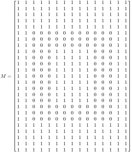
Singular value decompositions can be used to represent data efficiently. Suppose, for instance, that we wish to transmit the following image, which consists of an array of $15\times 25$ black or white pixels.
奇异值分解可用于高效表示数据。例如，假设我们需要传输一幅由 $15\times 25$ 个黑白像素组成的图像（如下所示）。

Since there are only three types of columns in this image, as shown below, it should be possible to represent the data in a more compact form.
观察图像可知，其列向量仅包含三种类型（如下图所示），因此我们可以用更紧凑的形式存储数据。

We will represent the image as a $15\times 25$ matrix in which each entry is either a $0$ (representing a black pixel) or $1$ (representing white). As such, there are $375$ entries in the matrix.
我们将图像表示为一个 $15\times 25$ 的矩阵，其中每个元素为 $0$（代表黑色像素）或 $1$（代表白色像素）。该矩阵共包含 $375$ 个元素。

If we perform a singular value decomposition on $M$, we find there are only three non-zero singular values:
对矩阵 $M$ 进行奇异值分解后，我们发现仅存在三个非零奇异值：

${\sigma }_1=14.72$,
${\sigma }_2=5.22$,
${\sigma }_3=3.31$

Therefore, the matrix may be represented as
因此，矩阵 $M$ 可表示为：

$$M={\mathbf{u}}_1{\sigma }_1{\mathbf{v}}_1^T+{\mathbf{u}}_2{\sigma }_2{\mathbf{v}}_2^T+{\mathbf{u}}_3{\sigma }_3{\mathbf{v}}_3^T$$

This means that we have three vectors ${\mathbf{v}}_i$ (each with $15$ entries), three vectors ${\mathbf{u}}_i$ (each with $25$ entries), and three singular values ${\sigma }_i$. This implies that we may represent the matrix using only $123$ numbers rather than the $375$ that appear in the matrix. In this way, the singular value decomposition discovers the redundancy in the matrix and provides a format for eliminating it.
这意味着我们仅需存储：3 个长度为 $15$ 的向量 ${\mathbf{v}}_i$、3 个长度为 $25$ 的向量 ${\mathbf{u}}_i$，以及 3 个奇异值 ${\sigma }_i$。总数据量仅为 $3\times 15+3\times 25+3=123$ 个数值，远少于原始矩阵的 $375$ 个元素。通过这种方式，奇异值分解能够识别矩阵中的数据冗余，并提供消除冗余的方法。

Why are there only three non-zero singular values? Remember that the number of non-zero singular values equals the rank of the matrix. In this case, we see that there are three linearly independent columns in the matrix, which means that the rank will be three.
为什么仅存在三个非零奇异值？回顾前文结论：非零奇异值的个数等于矩阵的秩。在这个例子中，矩阵的列向量包含三个线性无关的类型，因此矩阵的秩为 3。

Noise reduction

降噪

The previous example showed how we can exploit a situation where many singular values are zero. Typically speaking, the large singular values point to where the interesting information is. For example, imagine we have used a scanner to enter this image into our computer. However, our scanner introduces some imperfections (usually called “noise”) in the image.
前面的例子展示了如何利用“多数奇异值为 0”的特性压缩数据。通常来说，较大的奇异值对应数据中的关键信息。例如，假设我们用扫描仪将图像输入计算机，但扫描仪会在图像中引入一些干扰（通常称为“噪声”）。

We may proceed in the same way: represent the data using a $15\times 25$ matrix and perform a singular value decomposition. We find the following singular values:
我们仍采用相同的方法：将带噪声的图像表示为 $15\times 25$ 的矩阵，并对其进行奇异值分解。得到的奇异值如下：

${\sigma }_1=14.15$,
${\sigma }_2=4.67$,
${\sigma }_3=3.00$,
${\sigma }_4=0.21$,
${\sigma }_5=0.19$,
…,
${\sigma }_{15}=0.05$

Clearly, the first three singular values are the most important—so we will assume that the others are due to the noise in the image and make the approximation
显然，前三个奇异值远大于其余奇异值，因此我们假设：较小的奇异值由噪声引起，并对矩阵进行如下近似：

$$M\approx {\mathbf{u}}_1{\sigma }_1{\mathbf{v}}_1^T+{\mathbf{u}}_2{\sigma }_2{\mathbf{v}}_2^T+{\mathbf{u}}_3{\sigma }_3{\mathbf{v}}_3^T$$

This leads to the following improved image.
近似后的矩阵对应的图像如下，噪声得到了明显抑制。

Noisy image 带噪声的图像	Improved image 改进后的图像

Data analysis

数据分析

Noise also arises anytime we collect data: no matter how good the instruments are, measurements will always have some error in them. If we remember the theme that large singular values point to important features in a matrix, it seems natural to use a singular value decomposition to study data once it is collected.
在数据收集过程中，噪声几乎无处不在：无论测量仪器多么精密，数据总会存在误差。若我们牢记“大奇异值对应矩阵关键特征”这一核心思想，那么在数据收集完成后，使用奇异值分解进行数据分析就成了自然的选择。

As an example, suppose that we collect some data as shown below:
例如，假设我们收集到如下所示的数据点：

We may take the data and put it into a matrix:
我们可以将这些数据整理为如下矩阵：

$-1.03$	$0.74$	$-0.02$	$0.51$	$-1.31$	$0.99$	$0.69$	$-0.12$	$-0.72$	$1.11$
$-2.23$	$1.61$	$-0.02$	$0.88$	$-2.39$	$2.02$	$1.62$	$-0.35$	$-1.67$	$2.46$

and perform a singular value decomposition. We find the singular values
对该矩阵进行奇异值分解后，得到的奇异值为：

${\sigma }_1=6.04$,
${\sigma }_2=0.22$

With one singular value so much larger than the other, it may be safe to assume that the small value of ${\sigma }_2$ is due to noise in the data and that this singular value would ideally be zero. In that case, the matrix would have rank one—meaning that all the data lies on the line defined by ${\mathbf{u}}_1$.
由于 ${\sigma }_1$ 远大于 ${\sigma }_2$，我们可以合理假设：${\sigma }_2$ 的小值由数据噪声引起，理想情况下 ${\sigma }_2=0$。此时矩阵的秩为 1，意味着所有数据点都近似分布在由 ${\mathbf{u}}_1$ 定义的直线上。

This brief example points to the beginnings of a field known as principal component analysis (PCA), a set of techniques that uses singular values to detect dependencies and redundancies in data.
这个简短的例子指出了一个被称为主成分分析（PCA）的领域的开端，PCA 正是一组利用奇异值来检测数据中的依赖关系和冗余的技术。

In a similar way, singular value decompositions can be used to detect groupings in data, which explains why singular value decompositions are being used in attempts to improve Netflix’s movie recommendation system. Ratings of movies you have watched allow a program to sort you into a group of others whose ratings are similar to yours. Recommendations may be made by choosing movies that others in your group have rated highly.
类似地，奇异值分解还可用于检测数据中的分组结构，这也解释了为何奇异值分解会被用于优化 Netflix 的电影推荐系统。系统会根据你对已观看电影的评分，将你归入“评分偏好相似”的用户群体；之后，通过筛选该群体中其他用户高分评价的电影，即可为你生成推荐列表。

Summary

总结

As mentioned at the beginning of this article, the singular value decomposition should be a central part of an undergraduate mathematics major’s linear algebra curriculum. Besides having a rather simple geometric explanation, the singular value decomposition offers extremely effective techniques for putting linear algebraic ideas into practice. All too often, however, a proper treatment in an undergraduate linear algebra course seems to be missing.
正如本文开篇所述，奇异值分解应成为数学专业本科生线性代数课程的核心内容。它不仅具有简洁直观的几何解释，还能为线性代数思想的实际应用提供高效方法。然而，在许多本科线性代数课程中，奇异值分解的教学往往不够系统和深入。

This article has been somewhat impressionistic: I have aimed to provide some intuitive insights into the central idea behind singular value decompositions and then illustrate how this idea can be put to good use. More rigorous accounts may be readily found.
本文的阐述更偏向直观理解：核心目标是让读者掌握奇异值分解的核心思想，并了解其实际应用场景。若需更严谨的理论推导，相关资料并不难获取。

References:

参考文献：

• Gilbert Strang, Linear Algebra and Its Applications. Brooks Cole.
  Strang’s book is something of a classic though some may find it to be a little too formal.

• William H. Press et al, Numerical Recipes in C: The Art of Scientific Computing. Cambridge University Press.
  Authoritative, yet highly readable. Older versions are available online.

• Dan Kalman, A Singularly Valuable Decomposition: The SVD of a Matrix, The College Mathematics Journal 27 (1996), 2-23.
  Kalman’s article, like this one, aims to improve the profile of the singular value decomposition. It also includes a description of how least-squares computations are facilitated by the decomposition.

• If You Liked This, You’re Sure to Love That, The New York Times, November 21, 2008.
  This article describes Netflix’s prize competition as well as some of the challenges associated with it.

---

via：

• We Recommend a Singular Value Decomposition - AMS :: Feature Column from the AMS, Posted August 2009.
  https://www.ams.org/publicoutreach/feature-column/fcarc-svd