ML4T - 第7章第5节 用线性回归预测股票回报Prediction stock returns with linear regression

目录

一、Load Data 加载数据

二、Custom MultipleTimeSeriesCV 自定义时间序列交叉验证

三、Visualization helper functions 可视化辅助函数

四、Linear Regression with sklearn 线性回归模型

五、Linear Regression、Ridge Regression、Lasso Regression模型对比

六、Ridge Regression 岭回归

七、Lasso Regression 套索回归

八、Compare results 对比模型

---

一、Load Data 加载数据

这里只选取 成交额前100名的数据进行分析（需要按照前面的帖子获取原始数据）

we select top 100 of data.dollar_vol_rank to analyse.

data = data[data.dollar_vol_rank<100]

import warnings
warnings.filterwarnings('ignore')%matplotlib inlinefrom time import time
from pathlib import Path
import pandas as pd
import numpy as np
from scipy.stats import spearmanrfrom sklearn.metrics import mean_squared_error
from sklearn.preprocessing import StandardScaler
from sklearn.linear_model import LinearRegression, Ridge, Lasso
from sklearn.pipeline import Pipelineimport seaborn as sns
import matplotlib.pyplot as plt
from matplotlib.ticker import FuncFormattersns.set_style('darkgrid')
idx = pd.IndexSliceYEAR = 252with pd.HDFStore('data.h5') as store:data = (store['model_data'].dropna().drop(['open', 'close', 'low', 'high'], axis=1))data.index.names = ['symbol', 'date']
data = data.drop([c for c in data.columns if 'lag' in c], axis=1)# Select Investment Universe 选择投资范围
data = data[data.dollar_vol_rank<100]# Create Model Data  创建模型数据
y = data.filter(like='target')
X = data.drop(y.columns, axis=1)
X = X.drop(['dollar_vol', 'dollar_vol_rank', 'volume', 'consumer_durables'], axis=1)# data.info(null_counts=True)
data.info(show_counts=True)

<class 'pandas.core.frame.DataFrame'>
MultiIndex: 109434 entries, ('AAL', Timestamp('2013-07-26 00:00:00')) to ('YUM', Timestamp('2015-11-03 00:00:00'))
Data columns (total 45 columns):#   Column                 Non-Null Count   Dtype  
---  ------                 --------------   -----  0   volume                 109434 non-null  float641   dollar_vol             109434 non-null  float642   dollar_vol_1m          109434 non-null  float643   dollar_vol_rank        109434 non-null  float644   rsi                    109434 non-null  float645   bb_high                109434 non-null  float646   bb_low                 109434 non-null  float647   atr                    109434 non-null  float648   macd                   109434 non-null  float649   return_1d              109434 non-null  float6410  return_5d              109434 non-null  float6411  return_10d             109434 non-null  float6412  return_21d             109434 non-null  float6413  return_42d             109434 non-null  float6414  return_63d             109434 non-null  float6415  target_1d              109434 non-null  float6416  target_5d              109434 non-null  float6417  target_10d             109434 non-null  float6418  target_21d             109434 non-null  float6419  year_2014              109434 non-null  bool   20  year_2015              109434 non-null  bool   21  year_2016              109434 non-null  bool   22  year_2017              109434 non-null  bool   23  month_2                109434 non-null  bool   24  month_3                109434 non-null  bool   25  month_4                109434 non-null  bool   26  month_5                109434 non-null  bool   27  month_6                109434 non-null  bool   28  month_7                109434 non-null  bool   29  month_8                109434 non-null  bool   30  month_9                109434 non-null  bool   31  month_10               109434 non-null  bool   32  month_11               109434 non-null  bool   33  month_12               109434 non-null  bool   34  capital_goods          109434 non-null  bool   35  consumer_durables      109434 non-null  bool   36  consumer_non-durables  109434 non-null  bool   37  consumer_services      109434 non-null  bool   38  energy                 109434 non-null  bool   39  finance                109434 non-null  bool   40  health_care            109434 non-null  bool   41  miscellaneous          109434 non-null  bool   42  public_utilities       109434 non-null  bool   43  technology             109434 non-null  bool   44  transportation         109434 non-null  bool   
dtypes: bool(26), float64(19)
memory usage: 19.8+ MB

二、Custom MultipleTimeSeriesCV 自定义时间序列交叉验证

这里其实只是将日期序列进行划分为训练集和测试集，后面再用时间结合原始数据得到新数据。

Here split train or test data by time, we get the date and then use them to build true data later.

class MultipleTimeSeriesCV:"""Generates tuples of train_idx, test_idx pairsAssumes the MultiIndex contains levels 'symbol' and 'date'purges overlapping outcomes"""# 这里其实只是将日期序列进行划分为训练集和测试集，后面再用时间结合原始数据得到新数据。def __init__(self,n_splits=3,train_period_length=126,test_period_length=21,lookahead=None,shuffle=False):self.n_splits = n_splitsself.lookahead = lookaheadself.test_length = test_period_lengthself.train_length = train_period_lengthself.shuffle = shuffledef split(self, X, y=None, groups=None):unique_dates = X.index.get_level_values('date').unique()days = sorted(unique_dates, reverse=True)split_idx = []for i in range(self.n_splits):test_end_idx = i * self.test_lengthtest_start_idx = test_end_idx + self.test_length# train_end_idx = test_start_idx + + self.lookahead - 1  # Maybe an extra plus sign 可能多加了+train_end_idx = test_start_idx + self.lookahead - 1train_start_idx = train_end_idx + self.train_length + self.lookahead - 1split_idx.append([train_start_idx, train_end_idx,test_start_idx, test_end_idx])dates = X.reset_index()[['date']]for train_start, train_end, test_start, test_end in split_idx:train_idx = dates[(dates.date > days[train_start])& (dates.date <= days[train_end])].indextest_idx = dates[(dates.date > days[test_start])& (dates.date <= days[test_end])].indexif self.shuffle:np.random.shuffle(list(train_idx))yield train_idx, test_idxdef get_n_splits(self, X, y, groups=None):return self.n_splits# Verify that it works 验证它是否有效
train_period_length = 63     # 3 months
test_period_length = 10      # 10 days
n_splits = int(3 * YEAR/test_period_length)  # 3 years
lookahead = 1                # 向前看1天cv = MultipleTimeSeriesCV(n_splits=n_splits,test_period_length=test_period_length,lookahead=lookahead,train_period_length=train_period_length)i = 0
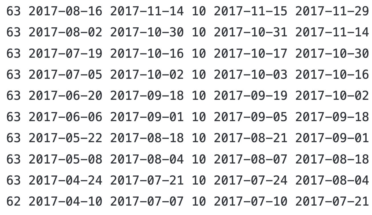
for train_idx, test_idx in cv.split(X=data):train = data.iloc[train_idx]train_dates = train.index.get_level_values('date')test = data.iloc[test_idx]test_dates = test.index.get_level_values('date')# df = train.reset_index().append(test.reset_index()) # baddf = pd.concat([train.reset_index(), test.reset_index()])  # pandas ≥ 2.0 goodn = len(df)assert n== len(df.drop_duplicates())print(train.groupby(level='symbol').size().value_counts().index[0],  # 一个train的fold有多少天数据train_dates.min().date(), train_dates.max().date(),            # 起止时间test.groupby(level='symbol').size().value_counts().index[0],test_dates.min().date(), test_dates.max().date())i += 1if i == 10:break

每一行：训练集的数量、开始时间、结束时间；测试集的数量、开始时间、结束时间

三、Visualization helper functions 可视化辅助函数

这是用来后面做图用的

# Prediction vs Actual Scatter Plot 预测与实际散点图
def plot_preds_scatter(df, ticker=None):if ticker is not None:idx = pd.IndexSlicedf = df.loc[idx[ticker, :], :]j = sns.jointplot(x='predicted', y='actuals',robust=True, ci=None,line_kws={'lw': 1, 'color': 'k'},scatter_kws={'s': 1},data=df,kind='reg')j.ax_joint.yaxis.set_major_formatter(FuncFormatter(lambda y, _: '{:.1%}'.format(y)))j.ax_joint.xaxis.set_major_formatter(FuncFormatter(lambda x, _: '{:.1%}'.format(x)))j.ax_joint.set_xlabel('Predicted')j.ax_joint.set_ylabel('Actuals')# Daily IC Distribution 每日IC(Information Coefficient 信息系数)分布
def plot_ic_distribution(df, ax=None):if ax is not None:sns.distplot(df.ic, ax=ax)else:ax = sns.distplot(df.ic)mean, median = df.ic.mean(), df.ic.median()ax.axvline(0, lw=1, ls='--', c='k')ax.text(x=.05, y=.9,s=f'Mean: {mean:8.2f}\nMedian: {median:5.2f}',horizontalalignment='left',verticalalignment='center',transform=ax.transAxes)ax.set_xlabel('Information Coefficient')sns.despine()plt.tight_layout()def plot_ic_distribution(df, ax=None):if ax is not None:sns.distplot(df.ic, ax=ax)else:ax = sns.distplot(df.ic)mean, median = df.ic.mean(), df.ic.median()ax.axvline(0, lw=1, ls='--', c='k')ax.text(x=.05, y=.9,s=f'Mean: {mean:8.2f}\nMedian: {median:5.2f}',horizontalalignment='left',verticalalignment='center',transform=ax.transAxes)ax.set_xlabel('Information Coefficient')sns.despine()plt.tight_layout()# Rolling Daily IC 滚动每日IC
def plot_rolling_ic(df):fig, axes = plt.subplots(nrows=2, sharex=True, figsize=(14, 8))rolling_result = df.sort_index().rolling(21).mean().dropna()mean_ic = df.ic.mean()rolling_result.ic.plot(ax=axes[0],title=f'Information Coefficient (Mean: {mean_ic:.2f})',lw=1)axes[0].axhline(0, lw=.5, ls='-', color='k')axes[0].axhline(mean_ic, lw=1, ls='--', color='k')mean_rmse = df.rmse.mean()rolling_result.rmse.plot(ax=axes[1],title=f'Root Mean Squared Error (Mean: {mean_rmse:.2%})',lw=1,ylim=(0, df.rmse.max()))axes[1].axhline(df.rmse.mean(), lw=1, ls='--', color='k')sns.despine()plt.tight_layout()

四、Linear Regression with sklearn 线性回归模型

这里可以简单理解为，用很多个变量，拟合OLS模型，去预测某个变量。

We use many variables to fit OLS model, then predict some variable.

接下来，用历史数据训练线性回归模型，预测未来1天的目标值（target_1d），并通过交叉验证评估模型的预测能力（用IC和RMSE指标）。

指标	含义
IC（Information Coefficient）	每天预测值与真实值的Spearman秩相关系数，衡量排序能力。越高越好，>5%算不错。
RMSE（Root Mean Squared Error）	每天预测值与真实值的均方根误差，衡量预测精度。越小越好。

lr_r, lr_p = spearmanr(lr_predictions.actuals, lr_predictions.predicted)
print(f'Information Coefficient (overall): {lr_r:.3%} (p-value: {lr_p:.4%})')

• 整体IC：把所有预测值和真实值拼在一起，计算一个总的Spearman相关系数。

• p-value：检验这个IC是否显著（<5%才算显著）。

• 如果这个IC是1.2%（p=12.3%），说明模型整体预测能力很弱，不显著。

%%time
# Set up cross-validation 交叉验证
train_period_length = 63
test_period_length = 10
n_splits = int(3 * YEAR / test_period_length)
lookahead = 1cv = MultipleTimeSeriesCV(n_splits=n_splits,test_period_length=test_period_length,lookahead=lookahead,train_period_length=train_period_length)# Run cross-validation with LinearRegression 运行线性回归模型的交叉验证target = f'target_{lookahead}d'
lr_predictions, lr_scores = [], []
lr = LinearRegression()
for i, (train_idx, test_idx) in enumerate(cv.split(X), 1):X_train, y_train, = X.iloc[train_idx], y[target].iloc[train_idx]X_test, y_test = X.iloc[test_idx], y[target].iloc[test_idx]lr.fit(X=X_train, y=y_train)y_pred = lr.predict(X_test)preds = y_test.to_frame('actuals').assign(predicted=y_pred)preds_by_day = preds.groupby(level='date')scores = pd.concat([preds_by_day.apply(lambda x: spearmanr(x.predicted,x.actuals)[0] * 100).to_frame('ic'),preds_by_day.apply(lambda x: np.sqrt(mean_squared_error(y_pred=x.predicted,y_true=x.actuals))).to_frame('rmse')], axis=1)lr_scores.append(scores)lr_predictions.append(preds)lr_scores = pd.concat(lr_scores)
lr_predictions = pd.concat(lr_predictions)# Persist results 保存
lr_scores.to_hdf('data.h5', 'lr/scores')
lr_predictions.to_hdf('data.h5', 'lr/predictions')
lr_scores = pd.read_hdf('data.h5', 'lr/scores')
lr_predictions = pd.read_hdf('data.h5', 'lr/predictions')# Evaluate results 评估结果
lr_r, lr_p = spearmanr(lr_predictions.actuals, lr_predictions.predicted)
print(f'Information Coefficient (overall): {lr_r:.3%} (p-value: {lr_p:.4%})')# Prediction vs Actuals Scatter 预测值与实际值散点图
plot_preds_scatter(lr_predictions)

结果：

Information Coefficient (overall): 1.346% (p-value: 0.0255%)
CPU times: user 23.7 s, sys: 2.9 s, total: 26.6 s
Wall time: 5.73 s

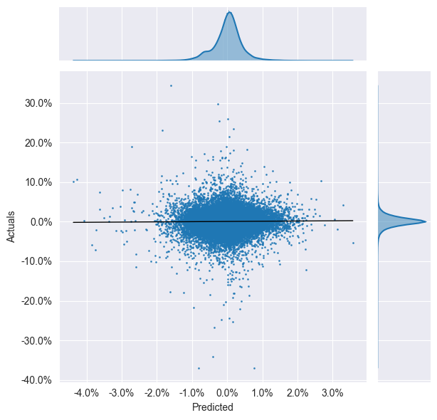
我的分析：

这个结果整体偏弱，虽然统计显著，但经济意义不强。

IC is too low, not good.

# Daily IC Distribution
plot_ic_distribution(lr_scores)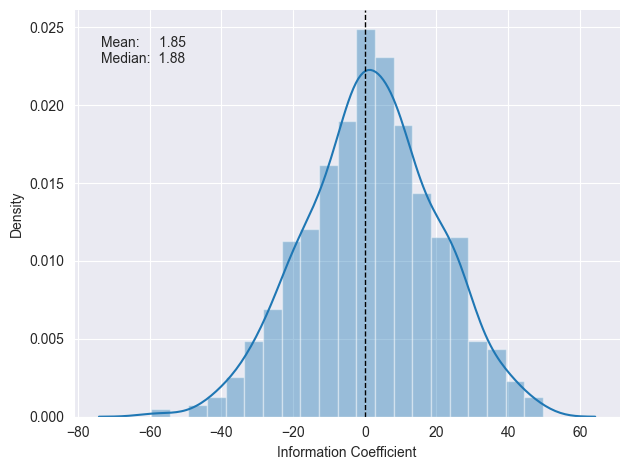

# Rolling Daily IC
plot_rolling_ic(lr_scores)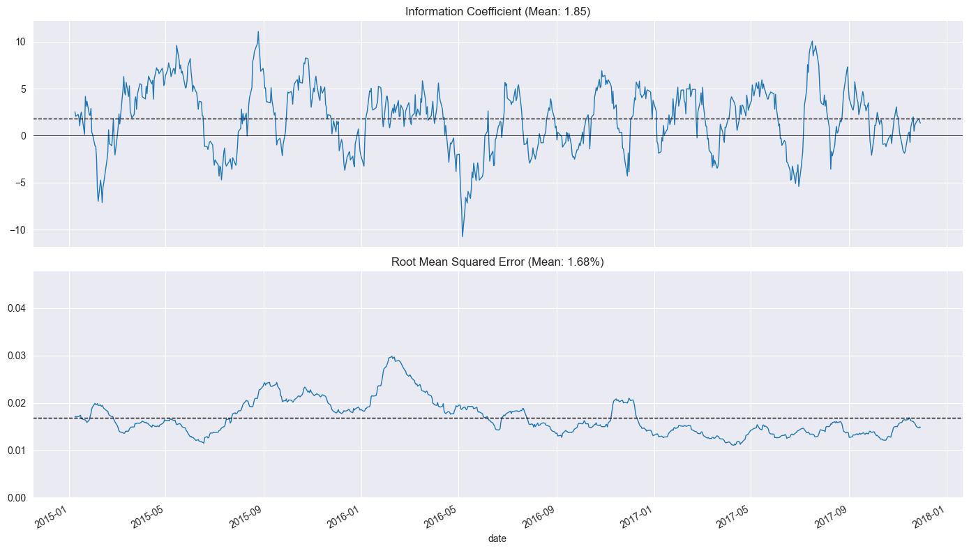

五、Linear Regression、Ridge Regression、Lasso Regression模型对比

因为我们后面还需要用到不同其他模型，所以这里我新增了一些对比知识。

英文	规范中文名	又常见叫法
Linear Regression	线性回归	普通最小二乘回归、OLS 回归
Ridge Regression	岭回归	吉洪诺夫正则化、L2 正则回归
Lasso Regression	套索回归	L1 正则回归、最小绝对值压缩选择算子

• “套索”是 LASSO acronym（Least Absolute Shrinkage and Selection Operator）的音意合译，形象地表示“把无用变量套走”。

这三者都属于线性模型，核心区别在损失函数里有没有“惩罚项”，也就是对系数大小的约束。

模型	关键词	本质区别
Linear Regression	无惩罚	最小化残差平方和，系数无约束，容易过拟合
Ridge Regression	L2 惩罚	在损失函数里加 λ·Σβ²，让系数变小但不归零，解决多重共线性
Lasso Regression	L1 惩罚	加 λ·Σβ，能把无用特征的系数压到 0，实现自动特征选择

• Linear Regression：解是最小二乘点，系数随便长。

• Ridge：解被拉向原点，圆约束 ⇒ 系数变小但非零。

• Lasso：解被拉向原点，菱形约束 ⇒ 顶点在坐标轴上 ⇒ 某些系数=0。

六、Ridge Regression 岭回归

在用时间序列交叉验证方式，遍历18个 Ridge 正则化强度 alpha，评估每个 alpha 下模型的预测能力（IC 和 RMSE），并记录模型系数，为后续选择最优 alpha 提供依据。

Using time series cross-validation, we evaluated the predictive performance (IC and RMSE) of the model for each of the 18 Ridge regularization strengths, denoted as alpha. We also recorded the model coefficients to inform the subsequent selection of the optimal alpha.

# %%time
# 在用时间序列交叉验证方式，遍历18个 Ridge 正则化强度 alpha，评估每个 alpha 下模型的预测能力（IC 和 RMSE），并记录模型系数，为后续选择最优 alpha 提供依据。
# Define cross-validation parameters
ridge_alphas = np.logspace(-4, 4, 9)
ridge_alphas = sorted(list(ridge_alphas) + list(ridge_alphas * 5))n_splits = int(3 * YEAR/test_period_length)
train_period_length = 63
test_period_length = 10
lookahead = 1cv = MultipleTimeSeriesCV(n_splits=n_splits,test_period_length=test_period_length,lookahead=lookahead,train_period_length=train_period_length)# Run cross-validation
target = f'target_{lookahead}d'X = X.drop([c for c in X.columns if 'year' in c], axis=1)ridge_coeffs, ridge_scores, ridge_predictions = {}, [], []for alpha in ridge_alphas:print(alpha, end=' ', flush=True)start = time()model = Ridge(alpha=alpha,fit_intercept=False,random_state=42)pipe = Pipeline([('scaler', StandardScaler()),('model', model)])coeffs = []for i, (train_idx, test_idx) in enumerate(cv.split(X), 1):X_train, y_train, = X.iloc[train_idx], y[target].iloc[train_idx]X_test, y_test = X.iloc[test_idx], y[target].iloc[test_idx]pipe.fit(X=X_train, y=y_train)y_pred = pipe.predict(X_test)preds = y_test.to_frame('actuals').assign(predicted=y_pred)preds_by_day = preds.groupby(level='date')scores = pd.concat([preds_by_day.apply(lambda x: spearmanr(x.predicted,x.actuals)[0] * 100).to_frame('ic'),preds_by_day.apply(lambda x: np.sqrt(mean_squared_error(y_pred=x.predicted,y_true=x.actuals))).to_frame('rmse')], axis=1)ridge_scores.append(scores.assign(alpha=alpha))ridge_predictions.append(preds.assign(alpha=alpha))coeffs.append(pipe.named_steps['model'].coef_)ridge_coeffs[alpha] = np.mean(coeffs, axis=0)print('\n')

Evaluate Ridge Results 评估

# Persist results
ridge_scores = pd.concat(ridge_scores)
ridge_scores.to_hdf('data.h5', 'ridge/scores')ridge_coeffs = pd.DataFrame(ridge_coeffs, index=X.columns).T
ridge_coeffs.to_hdf('data.h5', 'ridge/coeffs')ridge_predictions = pd.concat(ridge_predictions)
ridge_predictions.to_hdf('data.h5', 'ridge/predictions')ridge_scores = pd.read_hdf('data.h5', 'ridge/scores')
ridge_coeffs = pd.read_hdf('data.h5', 'ridge/coeffs')
ridge_predictions = pd.read_hdf('data.h5', 'ridge/predictions')# Evaluate Ridge Results
ridge_r, ridge_p = spearmanr(ridge_predictions.actuals, ridge_predictions.predicted)
print(f'Information Coefficient (overall): {ridge_r:.3%} (p-value: {ridge_p:.4%})')ridge_scores.groupby('alpha').ic.describe()

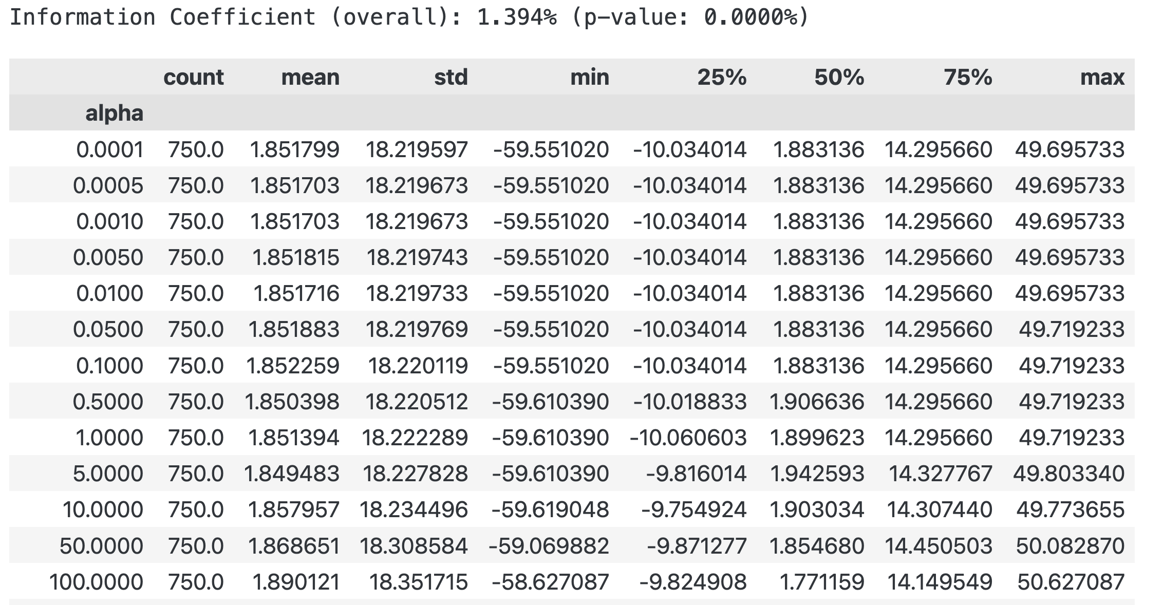
fig, axes = plt.subplots(ncols=2, sharex=True, figsize=(15, 5))scores_by_alpha = ridge_scores.groupby('alpha').ic.agg(['mean', 'median'])
best_alpha_mean = scores_by_alpha['mean'].idxmax()
best_alpha_median = scores_by_alpha['median'].idxmax()ax = sns.lineplot(x='alpha',y='ic',data=ridge_scores,estimator=np.mean,label='Mean',ax=axes[0])scores_by_alpha['median'].plot(logx=True,ax=axes[0],label='Median')axes[0].axvline(best_alpha_mean,ls='--',c='k',lw=1,label='Max. Mean')
axes[0].axvline(best_alpha_median,ls='-.',c='k',lw=1,label='Max. Median')
axes[0].legend()
axes[0].set_xscale('log')
axes[0].set_xlabel('Alpha')
axes[0].set_ylabel('Information Coefficient')
axes[0].set_title('Cross Validation Performance')ridge_coeffs.plot(logx=True,legend=False,ax=axes[1],title='Ridge Coefficient Path')axes[1].axvline(best_alpha_mean,ls='--',c='k',lw=1,label='Max. Mean')
axes[1].axvline(best_alpha_median,ls='-.',c='k',lw=1,label='Max. Median')
axes[1].set_xlabel('Alpha')
axes[1].set_ylabel('Coefficient Value')fig.suptitle('Ridge Results', fontsize=14)
sns.despine()
fig.tight_layout()
fig.subplots_adjust(top=.9)# 下面的左图：展示了不同 alpha 值下模型的 IC 分布。表示当alpha很大时效果变差了。
# 右图：展示了不同 alpha 值下模型的系数路径。表示当alpha很大时，模型的系数突然都变小了。

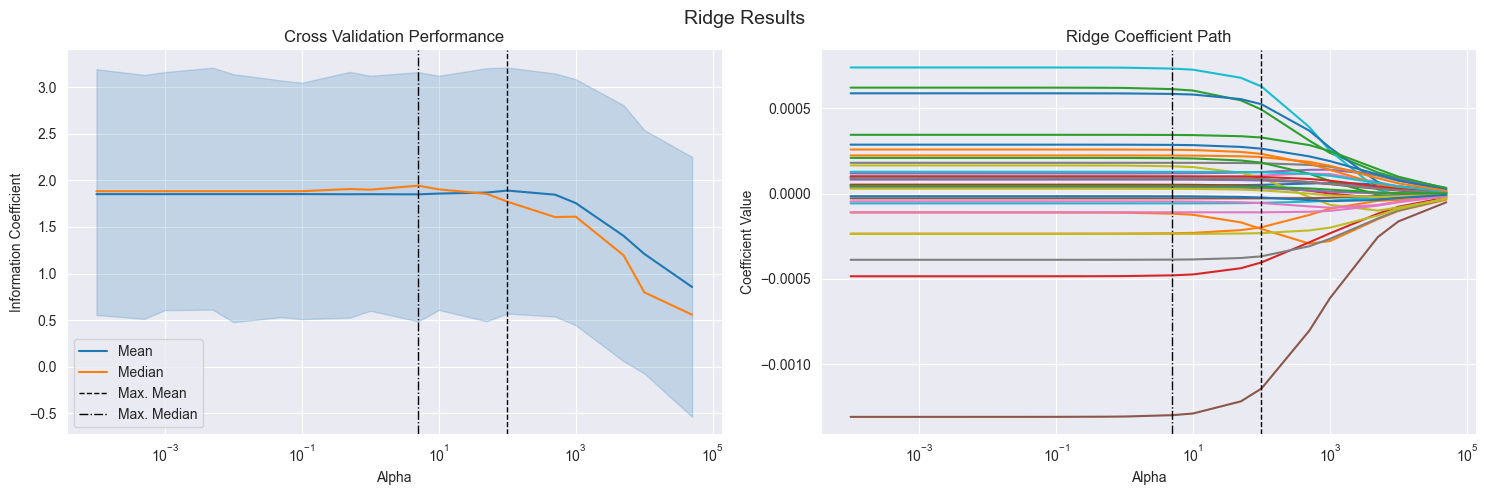
我的分析：

左图：展示了不同 alpha 值下模型的 IC 分布。表示当alpha很大时效果变差了。

右图：展示了不同 alpha 值下模型的系数路径。表示当alpha很大时，模型的系数突然都变小了。

# 只用最优 alpha 下的所有交叉验证折的结果
# 左图：如果分布集中在正值区域，说明模型大多数时候预测方向是对的。如果分布很宽、偏负，说明模型不稳定或信号弱。
# 右图：选出绝对值最大的10个特征，看哪些特征对预测贡献最大。best_alpha = ridge_scores.groupby('alpha').ic.mean().idxmax()
fig, axes = plt.subplots(ncols=2, figsize=(15, 5))
plot_ic_distribution(ridge_scores[ridge_scores.alpha == best_alpha],ax=axes[0])
axes[0].set_title('Daily Information Coefficients')
top_coeffs = ridge_coeffs.loc[best_alpha].abs().sort_values().head(10).index
top_coeffs.tolist()
ridge_coeffs.loc[best_alpha, top_coeffs].sort_values().plot.barh(ax=axes[1],title='Top 10 Coefficients')
sns.despine()
fig.tight_layout()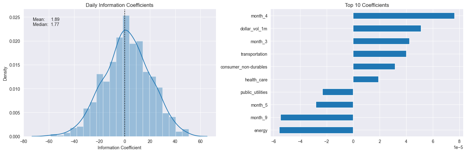

进一步分析：

左图：如果分布集中在正值区域，说明模型大多数时候预测方向是对的。如果分布很宽、偏负，说明模型不稳定或信号弱。
右图：选出绝对值最大的10个特征，看哪些特征对预测贡献最大。

plot_rolling_ic(ridge_scores[ridge_scores.alpha==best_alpha])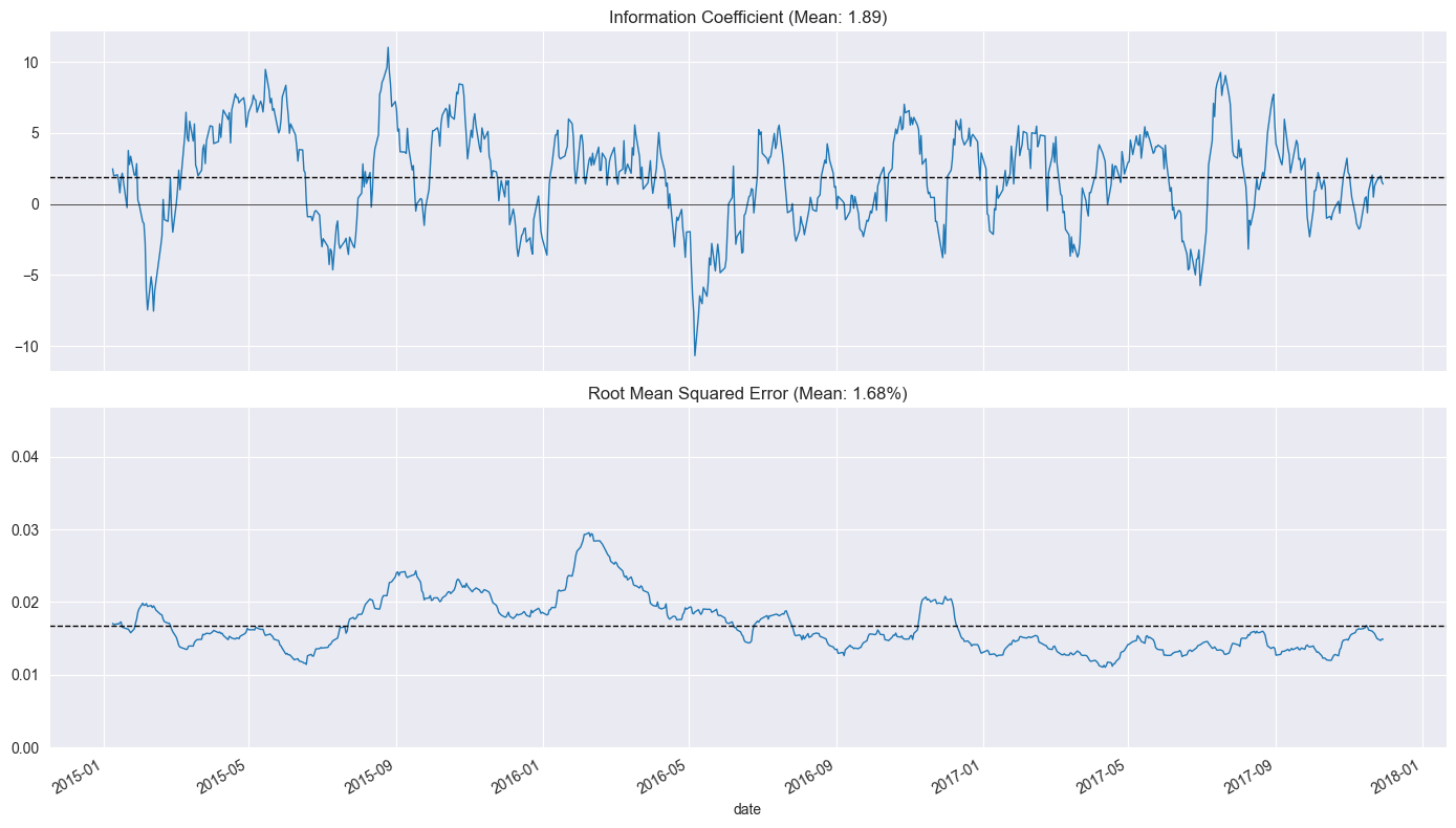

七、Lasso Regression 套索回归

和岭回归完全类似，

# 类似地
# Define cross-validation parameters
lasso_alphas = np.logspace(-10, -3, 8)train_period_length = 63
test_period_length = 10
YEAR = 252
n_splits = int(3 * YEAR / test_period_length) # three years
lookahead = 1cv = MultipleTimeSeriesCV(n_splits=n_splits,test_period_length=test_period_length,lookahead=lookahead,train_period_length=train_period_length)# Run cross-validation with Lasso regression
target = f'target_{lookahead}d'scaler = StandardScaler()
X = X.drop([c for c in X.columns if 'year' in c], axis=1)lasso_coeffs, lasso_scores, lasso_predictions = {}, [], []
for alpha in lasso_alphas:print(alpha, end=' ', flush=True)model = Lasso(alpha=alpha,fit_intercept=False,  # StandardScaler centers datarandom_state=42,tol=1e-3,max_iter=1000,warm_start=True,selection='random')pipe = Pipeline([('scaler', StandardScaler()),('model', model)])coeffs = []for i, (train_idx, test_idx) in enumerate(cv.split(X), 1):t = time()X_train, y_train, = X.iloc[train_idx], y[target].iloc[train_idx]X_test, y_test = X.iloc[test_idx], y[target].iloc[test_idx]pipe.fit(X=X_train, y=y_train)y_pred = pipe.predict(X_test)preds = y_test.to_frame('actuals').assign(predicted=y_pred)preds_by_day = preds.groupby(level='date')scores = pd.concat([preds_by_day.apply(lambda x: spearmanr(x.predicted,x.actuals)[0] * 100).to_frame('ic'),preds_by_day.apply(lambda x: np.sqrt(mean_squared_error(y_pred=x.predicted,y_true=x.actuals))).to_frame('rmse')],axis=1)lasso_scores.append(scores.assign(alpha=alpha))lasso_predictions.append(preds.assign(alpha=alpha))coeffs.append(pipe.named_steps['model'].coef_)lasso_coeffs[alpha] = np.mean(coeffs, axis=0)# Persist results
lasso_scores = pd.concat(lasso_scores)
lasso_scores.to_hdf('data.h5', 'lasso/scores')lasso_coeffs = pd.DataFrame(lasso_coeffs, index=X.columns).T
lasso_coeffs.to_hdf('data.h5', 'lasso/coeffs')lasso_predictions = pd.concat(lasso_predictions)
lasso_predictions.to_hdf('data.h5', 'lasso/predictions')

Evaluate Lasso Results 评估

best_alpha = lasso_scores.groupby('alpha').ic.mean().idxmax()
preds = lasso_predictions[lasso_predictions.alpha==best_alpha]lasso_r, lasso_p = spearmanr(preds.actuals, preds.predicted)
print(f'Information Coefficient (overall): {lasso_r:.3%} (p-value: {lasso_p:.4%})')lasso_scores.groupby('alpha').ic.agg(['mean', 'median'])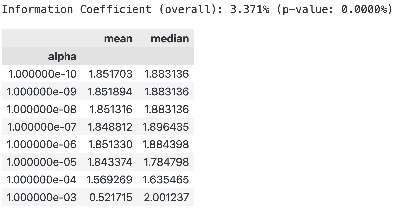

# Lasso Coefficient Path
fig, axes = plt.subplots(ncols=2, sharex=True, figsize=(15, 5))scores_by_alpha = lasso_scores.groupby('alpha').ic.agg(['mean', 'median'])
best_alpha_mean = scores_by_alpha['mean'].idxmax()
best_alpha_median = scores_by_alpha['median'].idxmax()# add code:
# Check if index is unique
print(lasso_scores.index.is_unique) # False表示索引不是唯一的
lasso_scores = lasso_scores.reset_index(drop=True)ax = sns.lineplot(x='alpha', y='ic', data=lasso_scores, estimator=np.mean, label='Mean', ax=axes[0])scores_by_alpha['median'].plot(logx=True, ax=axes[0], label='Median')axes[0].axvline(best_alpha_mean, ls='--', c='k', lw=1, label='Max. Mean')
axes[0].axvline(best_alpha_median, ls='-.', c='k', lw=1, label='Max. Median')
axes[0].legend()
axes[0].set_xscale('log')
axes[0].set_xlabel('Alpha')
axes[0].set_ylabel('Information Coefficient')
axes[0].set_title('Cross Validation Performance')lasso_coeffs.plot(logx=True, legend=False, ax=axes[1], title='Lasso Coefficient Path')
axes[1].axvline(best_alpha_mean, ls='--', c='k', lw=1, label='Max. Mean')
axes[1].axvline(best_alpha_median, ls='-.', c='k', lw=1, label='Max. Median')
axes[1].set_xlabel('Alpha')
axes[1].set_ylabel('Coefficient Value')fig.suptitle('Lasso Results', fontsize=14)
fig.tight_layout()
fig.subplots_adjust(top=.9)
sns.despine();

上面这段代码中，我们添加了：

# add code:

# Check if index is unique

print(lasso_scores.index.is_unique) # False表示索引不是唯一的

lasso_scores = lasso_scores.reset_index(drop=True)

否则可能不能正确执行。因为索引不唯一。

# Lasso IC Distribution and Top 10 Features
best_alpha = lasso_scores.groupby('alpha').ic.mean().idxmax()fig, axes = plt.subplots(ncols=2, figsize=(15, 5))
plot_ic_distribution(lasso_scores[lasso_scores.alpha==best_alpha], ax=axes[0])
axes[0].set_title('Daily Information Coefficients')top_coeffs = lasso_coeffs.loc[best_alpha].abs().sort_values().head(10).index
top_coeffs.tolist()
lasso_coeffs.loc[best_alpha, top_coeffs].sort_values().plot.barh(ax=axes[1], title='Top 10 Coefficients')sns.despine()
fig.tight_layout();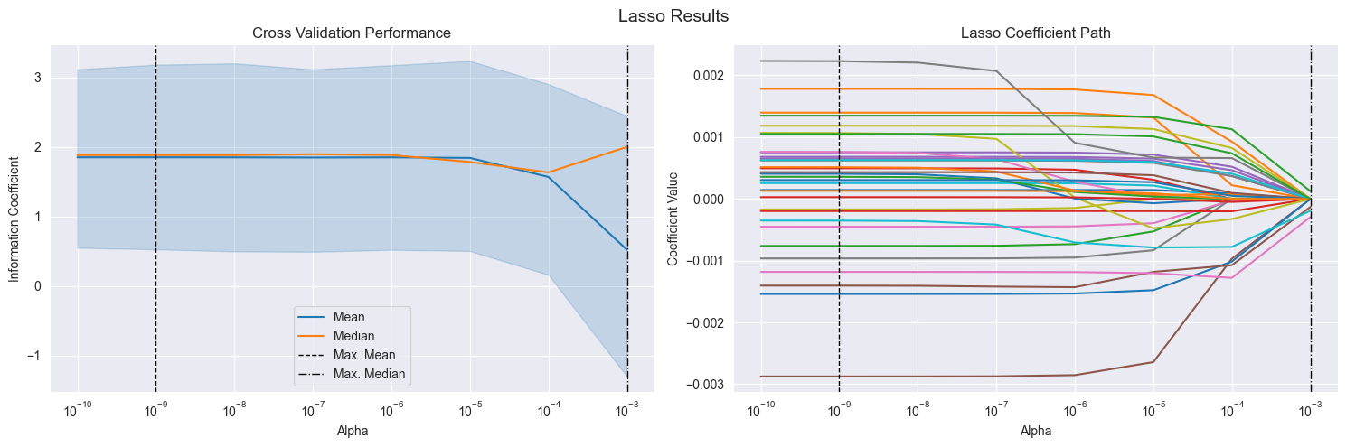

这里和原书作者结果有点不一样，感兴趣的可以参考原文：

https://github.com/stefan-jansen/machine-learning-for-trading/blob/main/07_linear_models/05_predicting_stock_returns_with_linear_regression.ipynb

# Lasso IC Distribution and Top 10 Features
best_alpha = lasso_scores.groupby('alpha').ic.mean().idxmax()fig, axes = plt.subplots(ncols=2, figsize=(15, 5))
plot_ic_distribution(lasso_scores[lasso_scores.alpha==best_alpha], ax=axes[0])
axes[0].set_title('Daily Information Coefficients')top_coeffs = lasso_coeffs.loc[best_alpha].abs().sort_values().head(10).index
top_coeffs.tolist()
lasso_coeffs.loc[best_alpha, top_coeffs].sort_values().plot.barh(ax=axes[1], title='Top 10 Coefficients')sns.despine()
fig.tight_layout();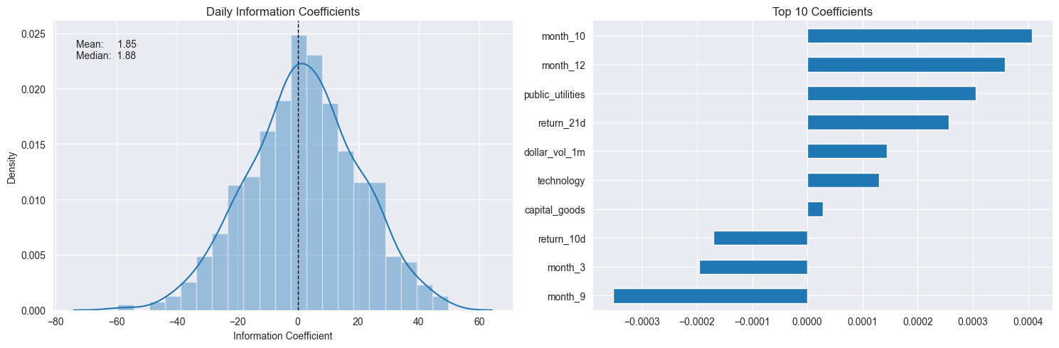

八、Compare results 对比模型

best_ridge_alpha = ridge_scores.groupby('alpha').ic.mean().idxmax()
best_ridge_preds = ridge_predictions[ridge_predictions.alpha==best_ridge_alpha]
best_ridge_scores = ridge_scores[ridge_scores.alpha==best_ridge_alpha]best_lasso_alpha = lasso_scores.groupby('alpha').ic.mean().idxmax()
best_lasso_preds = lasso_predictions[lasso_predictions.alpha==best_lasso_alpha]
best_lasso_scores = lasso_scores[lasso_scores.alpha==best_lasso_alpha]df = pd.concat([lr_scores.assign(Model='Linear Regression'),best_ridge_scores.assign(Model='Ridge Regression'),best_lasso_scores.assign(Model='Lasso Regression')]).drop('alpha', axis=1)
df.columns = ['IC', 'RMSE', 'Model']scores = df.groupby('Model').IC.agg(['mean', 'median'])
fig, axes = plt.subplots(ncols=2, figsize=(14,4), sharey=True, sharex=True)scores['mean'].plot.barh(ax=axes[0], xlim=(1.85, 2), title='Mean')
scores['median'].plot.barh(ax=axes[1], xlim=(1.8, 2.1), title='Median')
axes[0].set_xlabel('Daily IC')
axes[1].set_xlabel('Daily IC')fig.suptitle('Daily Information Coefficient by Model', fontsize=14)
sns.despine()
fig.tight_layout()
fig.subplots_adjust(top=.9)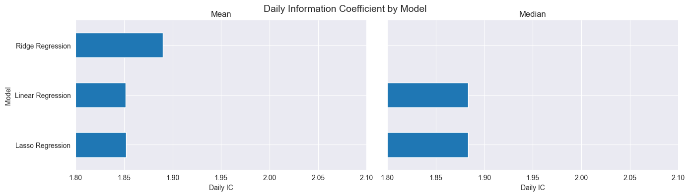

可以发现，基础版的线性回归效果不好时，可以试试成升级版的岭回归和套索回归。

Linear Regression IC is not the best(largest), we can try some other models.