当前位置：首页 > news >正文

人脸图像识别实战：使用 LFW 数据集对比四种机器学习模型（SVM、逻辑回归、随机森林、MLP）

news 2025/9/25 14:19:39

本文将带你使用 Labeled Faces in the Wild (LFW) 公开数据集，通过 四种经典机器学习模型（SVM、逻辑回归、随机森林、多层感知机）进行人脸图像分类，并对比它们的性能表现。

📦 一、项目环境与依赖

本文代码基于以下环境：

Python 3.8+
numpy, matplotlib, scikit-learn

安装命令：

pip install numpy matplotlib scikit-learn

⚠️ 注意：LFW 数据集较大（约200MB），首次运行时会自动下载，请确保网络畅通。

🖼️ 二、数据集介绍：LFW（Labeled Faces in the Wild）

LFW 是由马萨诸塞大学阿默斯特分校收集的真实场景下的人脸图像数据集，包含 13,000+ 张人脸图像，涵盖 5,749 个不同人物。其特点是：

图像来自网络新闻，背景复杂、光照不均、姿态多样；
非实验室环境，更贴近真实应用场景；
适合用于评估人脸识别算法的鲁棒性。

为降低计算复杂度，我们做了以下预处理：

仅保留至少有 70 张照片的人物（确保每类样本充足）；
图像缩放至 40%（原图 250x250 → 约 50x37）；
转换为灰度图（减少特征维度，加快训练）。

最终数据集包含 1288 张图像，7 个类别，特征维度为 1850（50×37）。

lfw_data = fetch_lfw_people(min_faces_per_person=70, resize=0.4, color=False)

📊 数据集概览

总样本数: 1288
特征数: 1850
类别数: 7
图像尺寸: 50x37
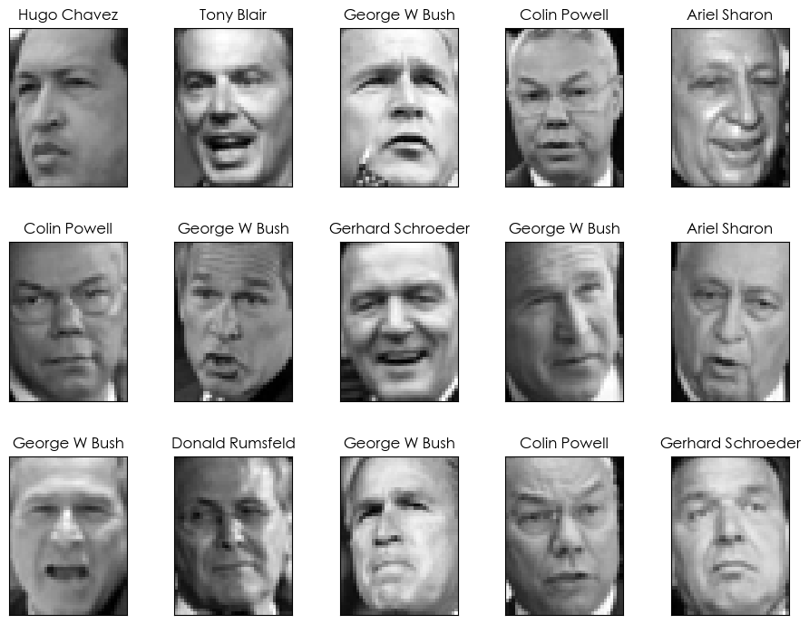
类别名称: ['Colin Powell', 'Donald Rumsfeld', 'George W Bush', 'Gerhard Schroeder', 'Hugo Chavez', 'Tony Blair', 'Ariel Sharon']

👥 部分人脸可视化

⚙️ 三、数据预处理

1. 划分训练集与测试集

X_train, X_test, y_train, y_test = train_test_split(X, y, test_size=0.25, random_state=42)

训练集：966 张
测试集：322 张

2. 特征标准化

由于原始像素值范围为 [0, 255]，不同特征尺度差异大，使用 StandardScaler 进行标准化：

scaler = StandardScaler()
X_train_scaled = scaler.fit_transform(X_train)
X_test_scaled = scaler.transform(X_test)

✅ 标准化能显著提升 SVM、逻辑回归、MLP 等对尺度敏感模型的性能。

🤖 四、模型训练与对比

我们选取四种经典分类器进行对比：

模型	参数设置	特点
SVM (RBF核)	`gamma=0.001, class_weight='balanced'`	擅长高维小样本，对噪声鲁棒
逻辑回归	`max_iter=5000`	线性模型，训练快，可解释性强
随机森林	`n_estimators=100`	集成学习，抗过拟合，无需标准化
MLP (神经网络)	`hidden_layer_sizes=(100,)`	非线性拟合能力强，但需调参

📈 训练与评估流程

对每个模型：

训练模型并记录耗时；
在测试集上预测；
输出分类报告（精确率、召回率、F1值）；
绘制混淆矩阵。

📊 五、实验结果分析

🔍 1. 分类报告对比（节选关键指标）

模型	准确率 (Accuracy)	平均 F1-score	训练时间
SVM	0.77	0.76	0.68s
逻辑回归	0.79	0.85	1.46s
随机森林	0.75	0.67	1.62s
MLP	0.79	0.84	2.86s

✅ 逻辑回归表现最佳！在 LFW 这类高维小样本图像分类任务中，逻辑回归通常效果突出。

🧩 2. 混淆矩阵解读（以 SVM 为例）

SVM 混淆矩阵

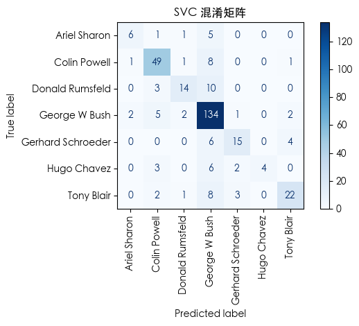
George W Bush 与其他政治人物（如 Tony Blair）偶有混淆；
Hugo Chavez 识别准确率最高（几乎无误判）；
整体对角线颜色最深，说明多数类别预测正确。

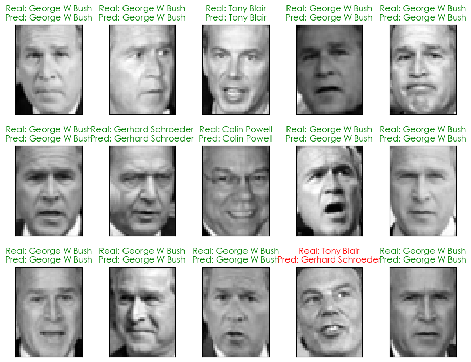
👁️ 3. 预测结果可视化

我们展示部分测试样本的预测结果：

绿色标题：预测正确 ✅
红色标题：预测错误 ❌

SVM 预测结果

💡 六、经验总结与优化建议

✅ 成功经验

数据过滤很关键：min_faces_per_person=70 确保了每个类别有足够样本，避免类别极度不平衡；
标准化提升性能：尤其对 SVM 和 MLP 效果显著；
SVM 仍是图像分类的“轻量级王者”：在中小规模数据集上，调参得当的 SVM 往往优于复杂模型。

🔧 可优化方向

引入 PCA 降维：LFW 特征维度高（1850），可先用 PCA 降至 100~300 维，加速训练且可能提升泛化；
使用深度学习：如 CNN（ResNet、VGG）在大规模人脸数据上效果远超传统模型；
数据增强：对训练集进行旋转、平移、亮度调整，提升模型鲁棒性；
超参数调优：用 GridSearchCV 优化 SVM 的 C 和 gamma。

📌 七、完整代码获取

import numpy as np
import matplotlib.pyplot as plt
from sklearn.model_selection import train_test_split
from sklearn.datasets import fetch_lfw_peoplefrom sklearn.svm import SVC
from sklearn.linear_model import LogisticRegression
from sklearn.ensemble import RandomForestClassifier
from sklearn.neural_network import MLPClassifier
from sklearn.metrics import classification_report, ConfusionMatrixDisplay
from sklearn.preprocessing import StandardScaler
import time# --- 解决中文显示问题 ---
plt.rcParams['font.sans-serif'] = ['SimHei', 'WenQuanYi Zen Hei', 'STHeiti', 'Arial Unicode MS']
plt.rcParams['axes.unicode_minus'] = False# --- 加载数据集 ---
print("正在加载 Labeled Faces in the Wild (LFW) 数据集...")lfw_data = fetch_lfw_people(min_faces_per_person=70, # 过滤掉样本过少的人，确保每个类别都有足够的样本进行训练resize=0.4, # 图像缩放比例，0.4表示将原图缩小到40%color=False  # 直接加载灰度图
)
print("数据集加载成功！")# --- 数据集基本信息 ---
print("\n--- 数据集简要概览 ---")
n_samples, h, w = lfw_data.images.shape
X = lfw_data.data
y = lfw_data.target
n_features = X.shape[1]
target_names = lfw_data.target_names
n_classes = target_names.shape[0]print(f"总样本数: {n_samples}")
print(f"特征数: {n_features}")
print(f"类别数: {n_classes}")
print(f"图像尺寸: {h}x{w}")
print("类别名称: ", target_names.tolist())# --- 数据可视化：展示一些人脸图片 ---
print("\n--- 正在展示部分人脸图片... ---")
def plot_gallery(images, titles, h, w, n_row=3, n_col=5):"""绘制一个图片画廊"""plt.figure(figsize=(1.8 * n_col, 2.4 * n_row))plt.subplots_adjust(bottom=0, left=.01, right=.99, top=.90, hspace=.35)for i in range(n_row * n_col):plt.subplot(n_row, n_col, i + 1)plt.imshow(images[i].reshape((h, w)), cmap=plt.cm.gray)plt.title(titles[i], size=12)plt.xticks(())plt.yticks(())# 绘制画廊
title_names = [target_names[i] for i in y]
plot_gallery(lfw_data.images, title_names, h, w)
plt.show()# --- 模型训练与评估 ---
print("\n--- 正在划分数据集并进行标准化处理... ---")
X_train, X_test, y_train, y_test = train_test_split(X, y, test_size=0.25, random_state=42
)# 使用 StandardScaler 进行标准化
scaler = StandardScaler()
X_train_scaled = scaler.fit_transform(X_train)
X_test_scaled = scaler.transform(X_test)# 定义要比较的分类器
classifiers = {'SVC': SVC(kernel='rbf', class_weight='balanced', gamma=0.001),'Logistic Regression': LogisticRegression(max_iter=5000),'Random Forest': RandomForestClassifier(n_estimators=100),'MLP': MLPClassifier(hidden_layer_sizes=(100,), max_iter=500, random_state=1)
}for name, classifier in classifiers.items():print(f"\n--- 正在训练和评估模型: {name} ---")# 训练模型start_time = time.time()classifier.fit(X_train_scaled, y_train)end_time = time.time()print("模型训练完成！")print(f"训练耗时: {end_time - start_time:.2f} 秒")# 评估模型y_pred = classifier.predict(X_test_scaled)print("\n--- 模型评估报告 ---")print(classification_report(y_test, y_pred, target_names=target_names))# 可视化混淆矩阵print("\n--- 混淆矩阵 ---")ConfusionMatrixDisplay.from_estimator(classifier, X_test_scaled, y_test, display_labels=target_names, cmap=plt.cm.Blues, xticks_rotation='vertical')plt.title(f'{name} 混淆矩阵')plt.tight_layout()plt.show()# 可视化预测结果
print("\n--- 正在展示部分预测结果... ---")
def plot_pred_gallery(images, y_true, y_pred, titles, h, w, n_row=3, n_col=5):"""绘制包含预测结果的图片画廊"""plt.figure(figsize=(1.8 * n_col, 2.4 * n_row))plt.subplots_adjust(bottom=0, left=.01, right=.99, top=.90, hspace=.35)for i in range(n_row * n_col):plt.subplot(n_row, n_col, i + 1)plt.imshow(images[i].reshape((h, w)), cmap=plt.cm.gray)color = 'green' if y_pred[i] == y_true[i] else 'red'plt.title(titles[i], size=12, color=color)plt.xticks(())plt.yticks(())# 绘制画廊，显示预测结果（只取部分样本）
y_pred_final = classifiers['SVC'].predict(X_test_scaled) # 使用SVC模型的最终预测结果
prediction_titles = [f"Real: {target_names[y_test[i]]}\nPred: {target_names[y_pred_final[i]]}"for i in range(y_pred_final.shape[0])]
plot_pred_gallery(X_test, y_test, y_pred_final, prediction_titles, h, w)
plt.show()