【OpenGL】LearnOpenGL学习笔记25 - 法线贴图 NormalMap
上接:https://blog.csdn.net/weixin_44506615/article/details/151876995?spm=1001.2014.3001.5501
完整代码:https://gitee.com/Duo1J/learn-open-gl | https://github.com/Duo1J/LearnOpenGL
法线贴图 (NormalMap)
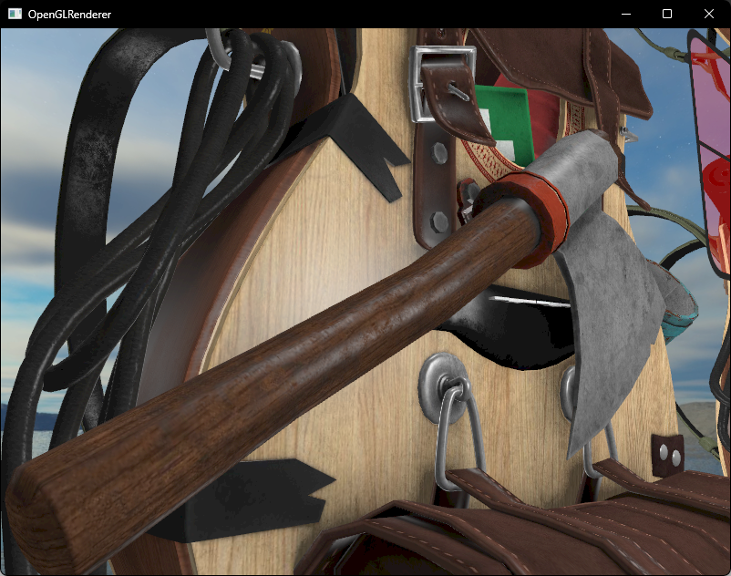
换回之前的背包场景,观察之前绘制的背包可以发现,模型的表面非常的平坦
比如斧头的木把手应该是粗糙不平的,可现在看起来很光滑
如果以光线的视角来看这个问题可以发现,表面之所以看起来这么平坦,是模型表面完全平行规整的法线导致的,如下图所示 (图片来自于LearnOpenGL)

所以要做出粗糙不平的效果,我们可以对每个片段所对应的法线进行改变,将这种改变的xyz坐标存储在纹理中的rgb通道,这样的问题就叫 法线贴图 (Normal Map) 或者 凹凸贴图 (Bump Map)
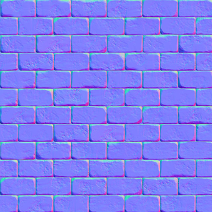
这是一个砖墙的法线贴图,可以看见其大部分都是偏蓝色的,这是因为所有法线的指向都是偏向Z轴的 (0, 0, 1)
在之前的背包资源文件夹中有一张背包的法线贴图,但我们不能直接对法线贴图进行采样然后应用法线,这是因为我们的法向量是处于世界空间,它不总是Z轴垂直于表面,所以我们需要进行空间变换,这会引用一个新的空间:切线空间
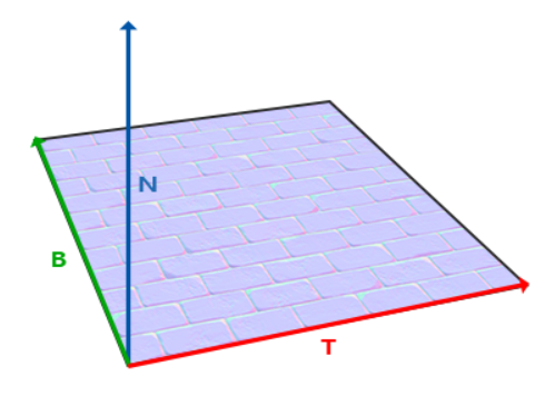
切线空间
切线空间是位于三角形表面上的空间,其法线永远指向正Z方向,另外两个轴为T (切线 Tangent)、B (副切线 Bitangent),加上 N (法线 Normal) 共称 TBN
 对于简单物体我们可以自行计算TBN,但对于较为复杂的物体计算较为麻烦,之前加载模型使用的Assimp库可以帮我们来计算切线,接下来修改一下之前的Model、Mesh、Vertex、Texture类
Vertex.h
增加切线和副切线,由于后续绑定顶点时需要连续的结构,这里需要注意顺序
#pragma once#include <glm.hpp>/**
* 顶点
*/
struct Vertex
{/*** 位置*/glm::vec3 position;/*** 法向量*/glm::vec3 normal;/*** UV*/glm::vec2 texCoord;/*** 切线*/glm::vec3 tangent;/*** 副切线*/glm::vec3 bitangent;
};
Model.cpp
void Model::LoadModel(std::string path)
{// ...// aiProcess_CalcTangentSpace: 计算切线空间const aiScene* scene = importer.ReadFile(path, aiProcess_Triangulate | aiProcess_FlipUVs | aiProcess_CalcTangentSpace);// ...
}Mesh Model::ProcessMesh(aiMesh* mesh, const aiScene* scene)
{// ...// 切线、副切线if (mesh->HasTangentsAndBitangents()){vertex.tangent = glm::vec3(mesh->mTangents[i].x, mesh->mTangents[i].y, mesh->mTangents[i].z);vertex.bitangent = glm::vec3(mesh->mBitangents[i].x, mesh->mBitangents[i].y, mesh->mBitangents[i].z);}// ...// 加载材质和纹理if (mesh->mMaterialIndex >= 0){// ...// 加载法线贴图std::vector<Texture> normalMaps = LoadMaterialTextures(material, aiTextureType_HEIGHT, TextureType::NORMAL);textures.insert(textures.end(), normalMaps.begin(), normalMaps.end());}
}
Mesh.cpp
void Mesh::Draw(const Shader& shader, int instanceCnt)
{// ...unsigned int normalNum = 0;// ...else if (texture.type == TextureType::NORMAL){number = std::to_string(++normalNum);}
}void Mesh::CreateBuffer()
{// ...// 外部临时绑定了Instance Offset,先跳过3glEnableVertexAttribArray(4);glVertexAttribPointer(4, 3, GL_FLOAT, false, sizeof(Vertex), (void*)offsetof(Vertex, tangent));glEnableVertexAttribArray(5);glVertexAttribPointer(5, 3, GL_FLOAT, false, sizeof(Vertex), (void*)offsetof(Vertex, bitangent));
}
Texture.cpp
std::string Texture::GetTypeName()
{if (type == TextureType::DIFFUSE){return "tex_diffuse";}else if (type == TextureType::SPECULAR){return "tex_specular";}else if (type == TextureType::NORMAL){return "tex_normal";}else{assert(false);return "";}
}
切线空间准备完毕,接下来可以开始应用法线贴图了
应用法线贴图
对于切线空间的转换有两种路径,先来尝试第一种,将采样后的法线左乘TBN矩阵转换到世界空间来使用
VertexShader.glsl
#version 330 corelayout (location = 0) in vec3 aPos;
layout (location = 1) in vec3 aNormal;
layout (location = 2) in vec2 aTexCoords;
layout (location = 3) in vec3 offset;
// 切线
layout (location = 4) in vec3 aTangent;
// 副切线
layout (location = 5) in vec3 aBitangent;out vec3 FragPos;
out vec3 Normal;
out vec2 TexCoords;uniform mat4 model;
layout (std140) uniform Matrices
{mat4 view;mat4 projection;
};out VS_OUT {vec3 FragPos;vec3 Normal;vec2 TexCoords;// 输出TBN矩阵mat3 TBN;vec3 Debug;
} vs_out;void main()
{gl_Position = projection * view * model * vec4(aPos + offset, 1.0);FragPos = vec3(model * vec4(aPos + offset, 1.0));vs_out.FragPos = FragPos;Normal = mat3(transpose(inverse(model))) * aNormal;vs_out.Normal = Normal;TexCoords = aTexCoords;vs_out.TexCoords = aTexCoords;// 计算TBN矩阵vec3 T = normalize(vec3(model * vec4(aTangent,   0.0)));vec3 B = normalize(vec3(model * vec4(aBitangent, 0.0)));vec3 N = normalize(vec3(model * vec4(aNormal,    0.0)));vs_out.TBN = mat3(T, B, N);
}
FragmentShader.glsl
// ...
struct Material {sampler2D tex_diffuse1;sampler2D tex_diffuse2;// ...sampler2D tex_specular1;sampler2D tex_specular2;// ...// 增加法线贴图sampler2D tex_normal1;sampler2D tex_normal2;// ...float shininess;
};
// ...
in VS_OUT {vec3 FragPos;vec3 Normal;vec2 TexCoords;mat3 TBN;vec3 Debug;
} fs_in;
// ...
void main()
{// 采样法线贴图vec3 normal = texture(material.tex_normal1, fs_in.TexCoords).rgb;// [-1, 1]转换到[0, 1]normal = normalize(normal * 2 - 1);// 左乘TBN矩阵转换到世界空间normal = normalize(fs_in.TBN * normal);// ...
}
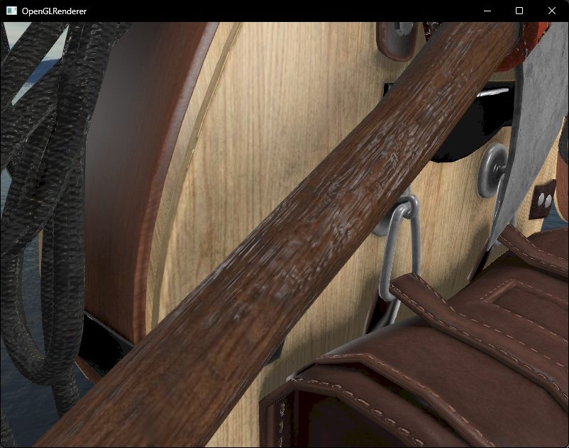
编译运行,可以发现木头把手有了凹凸不平的粗糙感
第二种方式则是反过来,我们使用TBN的逆矩阵将所有相关的世界空间向量转换为切线空间向量
VertexShader.glsl
// ...
out VS_OUT {vec3 FragPos;vec3 Normal;vec2 TexCoords;mat3 TBN;vec3 TangentViewPos;vec3 TangentFragPos;vec3 Debug;
} vs_out;
// ...
void main()
{// ...// 计算TBN矩阵vec3 T = normalize(vec3(model * vec4(aTangent,   0.0)));vec3 B = normalize(vec3(model * vec4(aBitangent, 0.0)));vec3 N = normalize(vec3(model * vec4(aNormal,    0.0)));// 这里不使用inverse是因为它是一个正交矩阵// 正交矩阵的逆矩阵和转置矩阵相等,但是transpose效率更高mat3 TBN = transpose(mat3(T, B, N));// 还是将TBN交给片段着色器用来计算lightPos,就先不移到顶点着色器了vs_out.TBN = TBN;vs_out.TangentViewPos  = TBN * viewPos;vs_out.TangentFragPos  = TBN * vec3(model * vec4(aPos + offset, 0.0));
}
FragmentShader.glsl
将用到的ViewPos、FragPos以及LightPos转换为切线空间向量
// 光照函数中的light.position改为
// normalize(fs_in.TBN * light.position)void main()
{// 采样法线贴图vec3 normal = texture(material.tex_normal1, fs_in.TexCoords).rgb;// [-1, 1]转换到[0, 1]normal = normalize(normal * 2 - 1);// 换为切线空间vec3 viewDir = normalize(fs_in.TangentViewPos - fs_in.TangentFragPos);// 平行光vec3 result = CalcDirectionalLight(dirLight, normal, viewDir);// 点光源for (int i = 0; i < POINT_LIGHT_NUM; i++){result += CalcPointLight(pointLight[i], normal, viewDir, fs_in.TangentFragPos);}FragColor = vec4(result, 1.0);
}
编译运行,我们可以看见和第一种方法一样的效果
但是这样我们将计算挪到了顶点着色器 (LightPos的转换也可以提前到顶点着色器进行),而通常顶点着色器运行次数会小于片段着色器,这会带来性能的提升
此外,还有一个问题和对应的技巧
当在更大的网格上计算切线向量的时候,它们往往有很大数量的共享顶点,当法向贴图应用到这些表面时将切线向量平均化通常能获得更好更平滑的结果。这样做有个问题,就是TBN向量可能会不能互相垂直,这意味着TBN矩阵不再是正交矩阵了。法线贴图可能会稍稍偏移。
我们可以使用叫做格拉姆-施密特正交化过程(Gram-Schmidt process)的数学技巧,我们可以对TBN向量进行重正交化,这样每个向量就又会重新垂直了。在顶点着色器中我们这样做:
vec3 T = normalize(vec3(model * vec4(tangent, 0.0)));
vec3 N = normalize(vec3(model * vec4(normal, 0.0)));
// re-orthogonalize T with respect to N
T = normalize(T - dot(T, N) * N);
// then retrieve perpendicular vector B with the cross product of T and N
vec3 B = cross(T, N);mat3 TBN = mat3(T, B, N)
完整代码可在顶部Git仓库中找到