第13周:LSTM实现糖尿病探索与预测
- 🍨 本文为🔗365天深度学习训练营 中的学习记录博客
- *🍖 参考:K同学啊
1.数据预处理
1.1硬件环境配置
import torch.nn as nn
import torch.nn.functional as F
import torchvision,torch

# 设置硬件设备,如果有GPU则使用,没有则使用cpu
device = torch.device("cuda" if torch.cuda.is_available() else "cpu")
device
device(type='cpu')
1.2数据导入
import numpy             as np
import pandas            as pd
import seaborn           as sns
from sklearn.model_selection   import train_test_split
import matplotlib.pyplot as plt
plt.rcParams['savefig.dpi'] = 500 #图片像素
plt.rcParams['figure.dpi']  = 500 #分辨率

plt.rcParams['font.sans-serif'] = ['SimHei']  # 用来正常显示中文标签

import warnings
warnings.filterwarnings("ignore")

DataFrame=pd.read_excel('./data/dia.xls')
DataFrame.head()
| 卡号 | 性别 | 年龄 | 高密度脂蛋白胆固醇 | 低密度脂蛋白胆固醇 | 极低密度脂蛋白胆固醇 | 甘油三酯 | 总胆固醇 | 脉搏 | 舒张压 | 高血压史 | 尿素氮 | 尿酸 | 肌酐 | 体重检查结果 | 是否糖尿病 | |
|---|---|---|---|---|---|---|---|---|---|---|---|---|---|---|---|---|
| 0 | 18054421 | 0 | 38 | 1.25 | 2.99 | 1.07 | 0.64 | 5.31 | 83 | 83 | 0 | 4.99 | 243.3 | 50 | 1 | 0 |
| 1 | 18054422 | 0 | 31 | 1.15 | 1.99 | 0.84 | 0.50 | 3.98 | 85 | 63 | 0 | 4.72 | 391.0 | 47 | 1 | 0 |
| 2 | 18054423 | 0 | 27 | 1.29 | 2.21 | 0.69 | 0.60 | 4.19 | 73 | 61 | 0 | 5.87 | 325.7 | 51 | 1 | 0 |
| 3 | 18054424 | 0 | 33 | 0.93 | 2.01 | 0.66 | 0.84 | 3.60 | 83 | 60 | 0 | 2.40 | 203.2 | 40 | 2 | 0 |
| 4 | 18054425 | 0 | 36 | 1.17 | 2.83 | 0.83 | 0.73 | 4.83 | 85 | 67 | 0 | 4.09 | 236.8 | 43 | 0 | 0 |
DataFrame.shape
(1006, 16)
1.3数据检查
# 查看数据是否有缺失值
print('数据缺失值---------------------------------')
print(DataFrame.isnull().sum())
数据缺失值---------------------------------
卡号            0
性别            0
年龄            0
高密度脂蛋白胆固醇     0
低密度脂蛋白胆固醇     0
极低密度脂蛋白胆固醇    0
甘油三酯          0
总胆固醇          0
脉搏            0
舒张压           0
高血压史          0
尿素氮           0
尿酸            0
肌酐            0
体重检查结果        0
是否糖尿病         0
dtype: int64
# 查看数据是否有重复值
print('数据重复值---------------------------------')
print('数据集的重复值为:'f'{DataFrame.duplicated().sum()}')
数据重复值---------------------------------
数据集的重复值为:0
1.4数据分析
# feature_map = {
# '年龄': '年龄',
# '高密度脂蛋白胆固醇': '高密度脂蛋白胆固醇',
# '低密度脂蛋白胆固醇': '低密度脂蛋白胆固醇',
# '极低密度脂蛋白胆固醇': '极低密度脂蛋白胆固醇',
# '甘油三酯': '甘油三酯',
# '总胆固醇': '总胆固醇',
# '脉搏': '脉搏',
# '舒张压':'舒张压',
# '高血压史':'高血压史',
# '尿素氮':'尿素氮',
# '尿酸':'尿酸',
# '肌酐':'肌酐',
# '体重检查结果':'体重检查结果'
# }
# plt.figure(figsize=(15, 10))
# for i, (col, col_name) in enumerate(feature_map.items(), 1):
# plt.subplot(3, 5, i)
# sns.boxplot(x=DataFrame['是否糖尿病'], y=DataFrame[col])
# plt.title(f'{col_name}的箱线图', fontsize=14)
# plt.ylabel('数值', fontsize=12)
# plt.grid(axis='y', linestyle='--', alpha=0.7)
# plt.tight_layout()
# plt.show()
import matplotlib.pyplot as plt
import seaborn as sns
# 创建一个新的图形,并设置其大小为15x10英寸
plt.figure(figsize=(15, 10))
# 遍历feature_map字典中的每个键值对
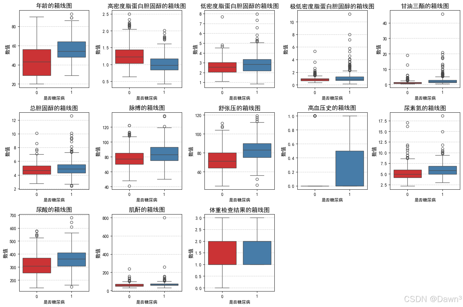
for i, (col, col_name) in enumerate(feature_map.items(), 1):
# 创建一个新的子图,该子图位于3行5列的网格的第i个位置
plt.subplot(3, 5, i)
# 创建一个箱线图,该图显示DataFrame中是否糖尿病列与当前特征列之间的关系
sns.boxplot(x=DataFrame['是否糖尿病'], y=DataFrame[col], palette="Set1")
# 设置当前子图的标题为当前特征的中文名称加上"的箱线图",字体大小为14
plt.title(f'{col_name}的箱线图', fontsize=14)
# 设置当前子图的y轴标签为"数值",字体大小为12
plt.ylabel('数值', fontsize=12)
# 在当前子图的y轴上添加网格线,线型为"--",透明度为0.7
plt.grid(axis='y', linestyle='--', alpha=0.7)
# 调整子图之间的间距,使得它们不会相互重叠
plt.tight_layout()
# 显示图形
plt.show()
1.5相关性分析
import plotly
import plotly.express as px

# 删除列 '卡号'
DataFrame.drop(columns=['卡号'], inplace=True)
# 计算各列之间的相关系数
df_corr = DataFrame.corr()

# 相关矩阵生成函数
def corr_generate(df):
    fig = px.imshow(df,text_auto=True,aspect="auto",color_continuous_scale='RdBu_r')
    fig.show()

# 生成相关矩阵
corr_generate(df_corr)

2.LSTM模型
2.1划分数据集
from sklearn.preprocessing import StandardScaler

# '高密度脂蛋白胆固醇'字段与糖尿病负相关,故而在 X 中去掉该字段
X = DataFrame.drop(['是否糖尿病','高密度脂蛋白胆固醇'],axis=1)
y = DataFrame['是否糖尿病']

# 数据集标准化处理
sc_X    = StandardScaler()
X = sc_X.fit_transform(X)

X = torch.tensor(np.array(X), dtype=torch.float32)
y = torch.tensor(np.array(y), dtype=torch.int64)

train_X, test_X, train_y, test_y = train_test_split(X, y,
                                                    test_size=0.2,
                                                    random_state=1)
train_X.shape, train_y.shape
(torch.Size([804, 13]), torch.Size([804]))
2.2数据集构建
from torch.utils.data import TensorDataset, DataLoader

train_dl = DataLoader(TensorDataset(train_X, train_y),
                      batch_size=64,
                      shuffle=False)

test_dl  = DataLoader(TensorDataset(test_X, test_y),
                      batch_size=64,
                      shuffle=False)
2.3定义模型
class model_lstm(nn.Module):
    def __init__(self):
        super(model_lstm, self).__init__()
        self.lstm0 = nn.LSTM(input_size=13 ,hidden_size=200,
                             num_layers=1, batch_first=True)

        self.lstm1 = nn.LSTM(input_size=200 ,hidden_size=200,
                             num_layers=1, batch_first=True)
        self.fc0   = nn.Linear(200, 2)

    def forward(self, x):

        out, hidden1 = self.lstm0(x)
        out, _ = self.lstm1(out, hidden1)
        out    = self.fc0(out)
        return out

model = model_lstm().to(device)
model
model_lstm(
  (lstm0): LSTM(13, 200, batch_first=True)
  (lstm1): LSTM(200, 200, batch_first=True)
  (fc0): Linear(in_features=200, out_features=2, bias=True)
)
3.训练模型
3.1定义训练函数
# 训练循环
def train(dataloader, model, loss_fn, optimizer):
    size = len(dataloader.dataset)  # 训练集的大小
    num_batches = len(dataloader)   # 批次数目, (size/batch_size,向上取整)

    train_loss, train_acc = 0, 0  # 初始化训练损失和正确率

    for X, y in dataloader:  # 获取图片及其标签
        X, y = X.to(device), y.to(device)

        # 计算预测误差
        pred = model(X)          # 网络输出
        loss = loss_fn(pred, y)  # 计算网络输出和真实值之间的差距,targets为真实值,计算二者差值即为损失

        # 反向传播
        optimizer.zero_grad()  # grad属性归零
        loss.backward()        # 反向传播
        optimizer.step()       # 每一步自动更新

        # 记录acc与loss
        train_acc  += (pred.argmax(1) == y).type(torch.float).sum().item()
        train_loss += loss.item()

    train_acc  /= size
    train_loss /= num_batches

    return train_acc, train_loss
3.2定义测试函数model
def test (dataloader, model, loss_fn):
    size        = len(dataloader.dataset)  # 测试集的大小
    num_batches = len(dataloader)          # 批次数目, (size/batch_size,向上取整)
    test_loss, test_acc = 0, 0

    # 当不进行训练时,停止梯度更新,节省计算内存消耗
    with torch.no_grad():
        for imgs, target in dataloader:
            imgs, target = imgs.to(device), target.to(device)

            # 计算loss
            target_pred = model(imgs)
            loss        = loss_fn(target_pred, target)

            test_loss += loss.item()
            test_acc  += (target_pred.argmax(1) == target).type(torch.float).sum().item()

    test_acc  /= size
    test_loss /= num_batches

    return test_acc, test_loss
3.3训练模型
loss_fn    = nn.CrossEntropyLoss() # 创建损失函数
learn_rate = 1e-4   # 学习率
opt        = torch.optim.Adam(model.parameters(),lr=learn_rate)
epochs     = 30

train_loss = []
train_acc  = []
test_loss  = []
test_acc   = []

for epoch in range(epochs):
    model.train()
    epoch_train_acc, epoch_train_loss = train(train_dl, model, loss_fn, opt)

    model.eval()
    epoch_test_acc, epoch_test_loss = test(test_dl, model, loss_fn)

    train_acc.append(epoch_train_acc)
    train_loss.append(epoch_train_loss)
    test_acc.append(epoch_test_acc)
    test_loss.append(epoch_test_loss)

    # 获取当前的学习率
    lr = opt.state_dict()['param_groups'][0]['lr']

    template = ('Epoch:{:2d}, Train_acc:{:.1f}%, Train_loss:{:.3f}, Test_acc:{:.1f}%, Test_loss:{:.3f}, Lr:{:.2E}')
    print(template.format(epoch+1, epoch_train_acc*100, epoch_train_loss,
                          epoch_test_acc*100, epoch_test_loss, lr))

print("="*20, 'Done', "="*20)
Epoch: 1, Train_acc:56.2%, Train_loss:0.686, Test_acc:53.0%, Test_loss:0.697, Lr:1.00E-04
Epoch: 2, Train_acc:56.2%, Train_loss:0.683, Test_acc:53.0%, Test_loss:0.697, Lr:1.00E-04
Epoch: 3, Train_acc:56.2%, Train_loss:0.679, Test_acc:53.0%, Test_loss:0.695, Lr:1.00E-04
Epoch: 4, Train_acc:56.3%, Train_loss:0.675, Test_acc:53.0%, Test_loss:0.693, Lr:1.00E-04
Epoch: 5, Train_acc:56.8%, Train_loss:0.670, Test_acc:54.0%, Test_loss:0.690, Lr:1.00E-04
Epoch: 6, Train_acc:57.6%, Train_loss:0.665, Test_acc:55.4%, Test_loss:0.685, Lr:1.00E-04
Epoch: 7, Train_acc:59.5%, Train_loss:0.658, Test_acc:56.4%, Test_loss:0.679, Lr:1.00E-04
Epoch: 8, Train_acc:61.1%, Train_loss:0.649, Test_acc:58.4%, Test_loss:0.671, Lr:1.00E-04
Epoch: 9, Train_acc:64.2%, Train_loss:0.638, Test_acc:62.4%, Test_loss:0.660, Lr:1.00E-04
Epoch:10, Train_acc:67.7%, Train_loss:0.622, Test_acc:63.9%, Test_loss:0.645, Lr:1.00E-04
Epoch:11, Train_acc:69.2%, Train_loss:0.595, Test_acc:66.3%, Test_loss:0.617, Lr:1.00E-04
Epoch:12, Train_acc:72.6%, Train_loss:0.547, Test_acc:70.3%, Test_loss:0.590, Lr:1.00E-04
Epoch:13, Train_acc:74.3%, Train_loss:0.510, Test_acc:69.8%, Test_loss:0.569, Lr:1.00E-04
Epoch:14, Train_acc:75.0%, Train_loss:0.489, Test_acc:70.3%, Test_loss:0.558, Lr:1.00E-04
Epoch:15, Train_acc:75.7%, Train_loss:0.476, Test_acc:72.3%, Test_loss:0.550, Lr:1.00E-04
Epoch:16, Train_acc:76.2%, Train_loss:0.466, Test_acc:72.8%, Test_loss:0.544, Lr:1.00E-04
Epoch:17, Train_acc:77.4%, Train_loss:0.458, Test_acc:72.8%, Test_loss:0.538, Lr:1.00E-04
Epoch:18, Train_acc:77.5%, Train_loss:0.451, Test_acc:72.8%, Test_loss:0.532, Lr:1.00E-04
Epoch:19, Train_acc:77.4%, Train_loss:0.445, Test_acc:72.8%, Test_loss:0.527, Lr:1.00E-04
Epoch:20, Train_acc:78.1%, Train_loss:0.440, Test_acc:72.8%, Test_loss:0.523, Lr:1.00E-04
Epoch:21, Train_acc:78.2%, Train_loss:0.435, Test_acc:72.8%, Test_loss:0.520, Lr:1.00E-04
Epoch:22, Train_acc:78.6%, Train_loss:0.430, Test_acc:72.3%, Test_loss:0.517, Lr:1.00E-04
Epoch:23, Train_acc:79.1%, Train_loss:0.426, Test_acc:72.3%, Test_loss:0.514, Lr:1.00E-04
Epoch:24, Train_acc:79.5%, Train_loss:0.423, Test_acc:72.3%, Test_loss:0.512, Lr:1.00E-04
Epoch:25, Train_acc:79.4%, Train_loss:0.419, Test_acc:72.8%, Test_loss:0.511, Lr:1.00E-04
Epoch:26, Train_acc:79.5%, Train_loss:0.416, Test_acc:73.3%, Test_loss:0.509, Lr:1.00E-04
Epoch:27, Train_acc:79.9%, Train_loss:0.413, Test_acc:74.3%, Test_loss:0.508, Lr:1.00E-04
Epoch:28, Train_acc:80.2%, Train_loss:0.410, Test_acc:74.3%, Test_loss:0.507, Lr:1.00E-04
Epoch:29, Train_acc:80.5%, Train_loss:0.408, Test_acc:74.3%, Test_loss:0.507, Lr:1.00E-04
Epoch:30, Train_acc:80.6%, Train_loss:0.405, Test_acc:75.2%, Test_loss:0.507, Lr:1.00E-04
==================== Done ====================
4.模型评估
4.1Loss与acc
import matplotlib.pyplot as plt
#隐藏警告
import warnings
warnings.filterwarnings("ignore")               #忽略警告信息
plt.rcParams['font.sans-serif']    = ['SimHei'] # 用来正常显示中文标签
plt.rcParams['axes.unicode_minus'] = False      # 用来正常显示负号
plt.rcParams['figure.dpi']         = 100        #分辨率

from datetime import datetime
current_time = datetime.now() # 获取当前时间

epochs_range = range(epochs)

plt.figure(figsize=(12, 3))
plt.subplot(1, 2, 1)

plt.plot(epochs_range, train_acc, label='Training Accuracy')
plt.plot(epochs_range, test_acc, label='Test Accuracy')
plt.legend(loc='lower right')
plt.title('Training and Validation Accuracy')
plt.xlabel(current_time) # 打卡请带上时间戳,否则代码截图无效

plt.subplot(1, 2, 2)
plt.plot(epochs_range, train_loss, label='Training Loss')
plt.plot(epochs_range, test_loss, label='Test Loss')
plt.legend(loc='upper right')
plt.title('Training and Validation Loss')
plt.show()
