极限平衡法和应力状态法无限坡模型安全系数计算

基于应力状态法的波致海底缓倾角无限坡滑动稳定性计算分析探讨——论文复现python程序代码

参考文献：
刘小丽：波致海底缓倾角无限坡滑动稳定性计算分析探讨
顾小芸：粘质海底稳定性实例分析

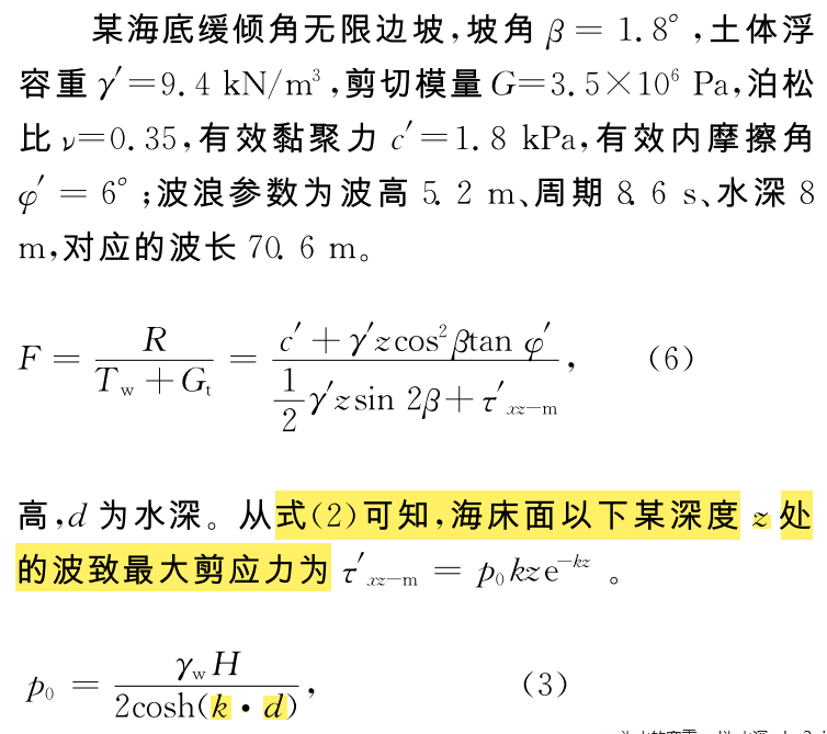
rw为水的容重，d为水深，k=2pi/L为波数，L为波长,z为海床面以下的深度
已知海水的密度ρ≈10094牛/m³

1. 极限平衡法

#角度要转换为弧度
beta=np.deg2rad(1.8);
gammap=9400;
G=3.5*10e6;
u=0.35;
cp=1800;
phip=np.deg2rad(6);
H=5.2;
T=8.6;
depth=8;
L=70.6;
rhow=10094
from __future__ import print_function, division
import numpy as np
import matplotlib as mpl
import matplotlib.pyplot as plt
%matplotlib inline
omega=1/T
#计算p0
p0=rhow*H/(2*np.cosh((2*np.pi)/L*depth))
print(p0)

20757.329154445302

#计算taopxz-m,计算海床面以下1.5m处的，z=1.5m
z=4
k=2*np.pi/L
taop=p0*k*z*np.exp(-k*z)
print(taop)

5176.10500297963

0.5*gammap*z*np.sin(2*beta)

1180.4617671510914

gammap*z*(np.cos(beta)**2)*np.tan(phip)

3948.020141038497

#计算F
F=(cp+gammap*z*(np.cos(beta)**2)*np.tan(phip))/(0.5*gammap*z*np.sin(2*beta)+taop)

print(F)

0.9042648884061498

封装函数

def FS_LIMIT(z,L,beta,gammap,cp,H,rhow,depth,phip):k=2*np.pi/Lp0=rhow*H/(2*np.cosh(k*depth))taop=p0*k*z*np.exp(-k*z)F=(cp+gammap*z*(np.cos(beta)**2)*np.tan(phip))/(0.5*gammap*z*np.sin(2*beta)+taop)return F

FS_LIMIT(z,L,beta,gammap,cp,H,rhow,depth,phip)

array([2.22448458, 1.40392622, 1.14407322, 1.02485479, 0.96226252,0.92829776, 0.91096398, 0.90426489, 0.90487034, 0.91078271,0.92073066, 0.93386596, 0.94960023, 0.96751162, 0.98728879,1.0086959 , 1.03154989, 1.05570539, 1.08104432, 1.10746866,1.13489523, 1.16325195, 1.19247502, 1.22250685, 1.25329451])

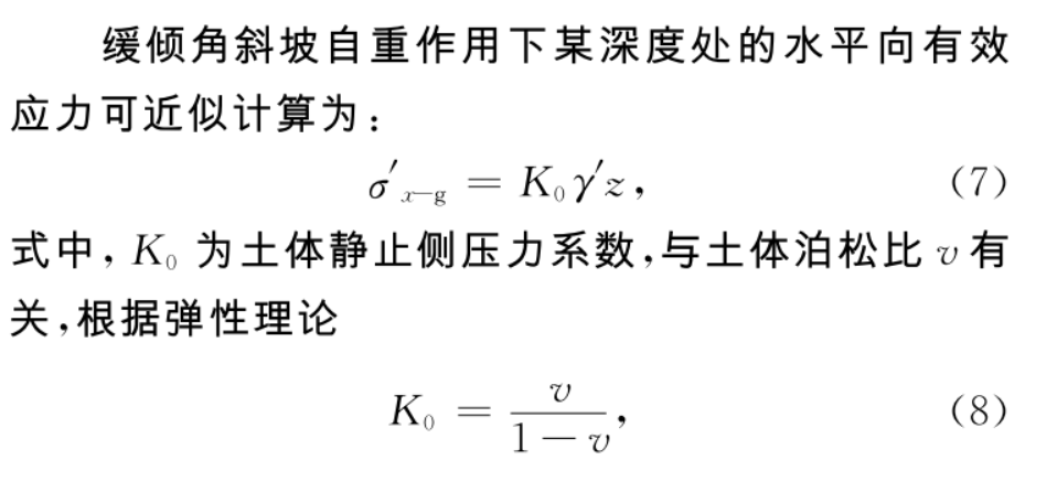
2. 应力状态法

#计算K0
K0=u/(1-u)
print(K0)

0.5384615384615384

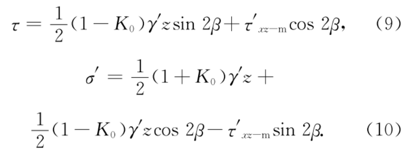
tao=0.5*(1-K0)*gammap*z*np.sin(2*beta)+taop*np.cos(2*beta)
segmap=0.5*(1+K0)*gammap*z+0.5*(1-K0)*gammap*z*np.cos(2*beta)-taop*np.sin(2*beta)
print(tao,segmap)

5710.719650040857 37257.867752086866

np.tan(phip)

0.10510423526567647

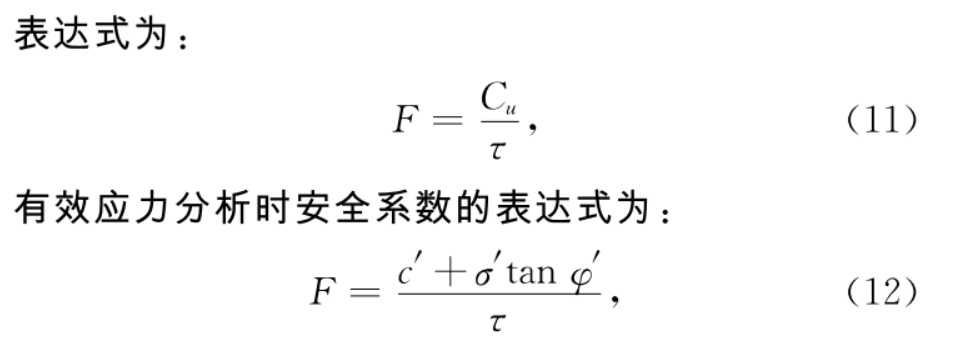
F_s=(cp+segmap*np.tan(phip))/tao
print(F_s)

1.0009175809693098

封装函数

def FS_STRESS(z,L,beta,gammap,cp,H,rhow,depth,phip,u):k=2*np.pi/Lp0=rhow*H/(2*np.cosh((2*np.pi)/L*depth))taop=p0*k*z*np.exp(-k*z)K0=u/(1-u)tao=0.5*(1-K0)*gammap*z*np.sin(2*beta)+taop*np.cos(2*beta)segmap=0.5*(1+K0)*gammap*z+0.5*(1-K0)*gammap*z*np.cos(2*beta)-taop*np.sin(2*beta)F=(cp+segmap*np.tan(phip))/taoreturn F

FS_STRESS(z,L,beta,gammap,cp,H,rhow,depth,phip,u)

1.0009175809693098

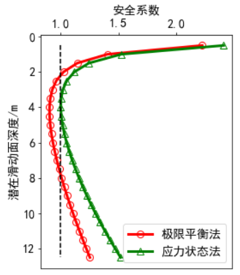
3. 计算z值变化时的结果——极限状态法和应力系数法对比

from __future__ import print_function, division
import numpy as np
import matplotlib as mpl
import matplotlib.pyplot as plt
plt.rcParams['font.family'] = ['sans-serif']
plt.rcParams['font.sans-serif'] = ['SimHei']
plt.rcParams['font.size'] =14
# %matplotlib inline
z=np.arange(0.5,13,0.5)
limit=np.zeros_like(z)
stress=np.zeros_like(z)
#角度要转换为弧度
beta=np.deg2rad(1.8);gammap=9400;G=3.5*10e6;u=0.35;cp=1800;phip=np.deg2rad(6);H=5.2;T=8.6;depth=8;L=70.6;rhow=10094;
fig,ax=plt.subplots(1,1,figsize=(4,5))
for i,j in enumerate(z):limit[i]=FS_LIMIT(j,L,beta,gammap,cp,H,rhow,depth,phip)stress[i]=FS_STRESS(j,L,beta,gammap,cp,H,rhow,depth,phip,u)
plt.plot(limit,z,'-ro',label='极限平衡法',lw=3,ms=8,mfc='none')
plt.plot(stress,z,'-g^',label='应力状态法',lw=3,ms=8,mfc='none')
plt.plot([1,1],[z.min(),z.max()],'--k')ax=plt.gca()
ax.xaxis.tick_top()
ax.invert_yaxis()
ax.set_title('安全系数',fontsize=14)
ax.set_ylabel('潜在滑动面深度/m')
plt.legend()
plt.show()
# fig.savefig(r'depth.svg',bbox_inches='tight')

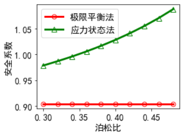
#z=4m，泊松比变化
from __future__ import print_function, division
import numpy as np
import matplotlib as mpl
import matplotlib.pyplot as plt
plt.rcParams['font.family'] = ['sans-serif']
plt.rcParams['font.sans-serif'] = ['SimHei']
plt.rcParams['font.size'] =14
# %matplotlib inline
u=np.arange(0.3,0.5,0.02)
limit=np.zeros_like(u)
stress=np.zeros_like(u)
#角度要转换为弧度
beta=np.deg2rad(1.8);gammap=9400;G=3.5*10e6;z=4;cp=1800;phip=np.deg2rad(6);H=5.2;T=8.6;depth=8;L=70.6;rhow=10094;
fig,ax=plt.subplots(1,1,figsize=(4,3))
for i,j in enumerate(u):limit[i]=FS_LIMIT(z,L,beta,gammap,cp,H,rhow,depth,phip)stress[i]=FS_STRESS(z,L,beta,gammap,cp,H,rhow,depth,phip,j)
plt.plot(u,limit,'-ro',label='极限平衡法',lw=3,ms=7,mfc='none')
plt.plot(u,stress,'-g^',label='应力状态法',lw=3,ms=8,mfc='none')
# ax=plt.gca()
# ax.xaxis.tick_top()
# ax.invert_yaxis()
plt.xlabel('泊松比')
plt.ylabel('安全系数')
plt.legend()
plt.show()
fig.savefig(r'possion ratio degree.svg',bbox_inches='tight')

#z=4m，坡度变化0.3~4
from __future__ import print_function, division
import numpy as np
import matplotlib as mpl
import matplotlib.pyplot as plt
plt.rcParams['font.family'] = ['sans-serif']
plt.rcParams['font.sans-serif'] = ['SimHei']
plt.rcParams['font.size'] =14
# %matplotlib inline
beta=np.arange(0.3,4,0.3)
limit=np.zeros_like(beta)
stress=np.zeros_like(beta)
#角度要转换为弧度
# beta=np.deg2rad(1.8);
gammap=9400;G=3.5*10e6;z=4;cp=1800;phip=np.deg2rad(6);H=5.2;T=8.6;depth=8;L=70.6;rhow=10094;u=0.35
fig,ax=plt.subplots(1,1,figsize=(4,3))
for i,j in enumerate(beta):limit[i]=FS_LIMIT(z,L,np.deg2rad(j),gammap,cp,H,rhow,depth,phip)stress[i]=FS_STRESS(z,L,np.deg2rad(j),gammap,cp,H,rhow,depth,phip,u)
plt.plot(beta,limit,'-ro',label='极限平衡法',lw=3,ms=7,mfc='none')
plt.plot(beta,stress,'-g^',label='应力状态法',lw=3,ms=8,mfc='none')
# ax=plt.gca()
# ax.xaxis.tick_top()
# ax.invert_yaxis()
plt.xlabel('坡角/°')
plt.ylabel('安全系数')
plt.legend()
plt.show()
fig.savefig(r'slope degree.svg',bbox_inches='tight')