疫菌QBD案例
本文是《A-VAX: Applying Quality by Design to Vaccines》第七个研究的R语言解决方案。
使用带两个中心点的二水平析因设计。运行10次实验。结果是分辨度为III的设计。
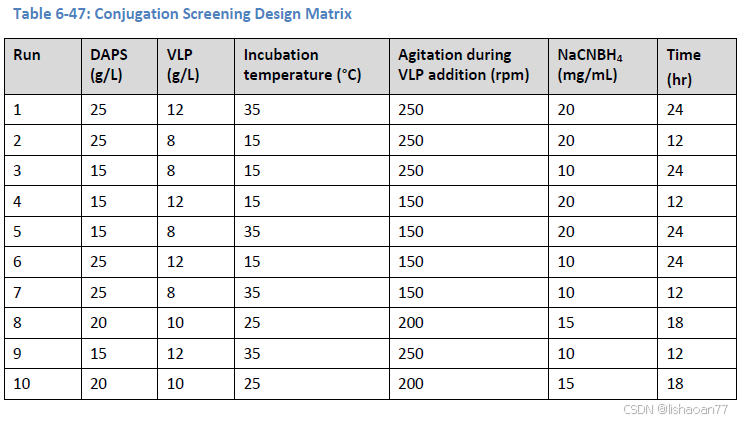
A <- c(25,25,15,15,15,25,25,20,15,20)
B <- c(12,8,8,12,8,12,8,10,12,10)
C <- c(35,15,15,15,35,15,35,25,35,25)
D <- c(250,250,250,150,150,150,150,200,250,200)
E <- c(20,20,10,20,20,10,10,15,10,15)
F <- c(24,12,24,12,24,24,12,18,12,18)
A <- c(1,1,-1,-1,-1,1,1,0,-1,0)
B <- c(1,-1,-1,1,-1,1,-1,0,1,0)
C <- c(1,-1,-1,-1,1,-1,1,0,1,0)
D <- c(1,1,1,-1,-1,-1,-1,0,1,0)
E <- c(1,1,-1,1,1,-1,-1,0,-1,0)
F <- c(1,-1,1,-1,1,1,-1,0,-1,0)
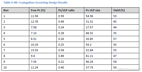
y1<-c(11.58,12.78,7.58,7.13,8.31,10.19,13.33,9.4,7.35,11.24)
y2<-c(0.59,0.49,0.24,0.28,0.26,0.25,0.58,0.49,0.22,0.40)
y3<-c(54.36,31.31,27.57,48.32,26.85,59.2,32.84,41.21,46.24,37.73)
y4<-c(53,45,44,35,57,35,53,47,58,56)
study6<- data.frame (A=A,B=B,C=C,D=D,E=E,F=F)
#aliases( lm( y1~ (.)^4, data = study6))
mod1 <- lm( y1 ~ (.), data = study6)
summary(mod1)
> summary(mod1)
Call:
lm.default(formula = y1 ~ (.), data = study6)
Residuals:
1 2 3 4 5 6 7 8 9 10
0.0160 -0.2315 0.0160 0.0160 -0.2315 -0.2315 0.0160 -0.4890 -0.2315 1.3510
Coefficients:
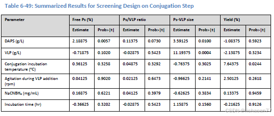
Estimate Std. Error t value Pr(>|t|)
(Intercept) 9.88900 0.27566 35.873 4.76e-05 ***
A 2.18875 0.30820 7.102 0.00574 **
B -0.71875 0.30820 -2.332 0.10195
C 0.36125 0.30820 1.172 0.32576
D 0.04125 0.30820 0.134 0.90200
E 0.16875 0.30820 0.548 0.62212
F -0.36625 0.30820 -1.188 0.32020
---
Signif. codes: 0 ‘***’ 0.001 ‘**’ 0.01 ‘*’ 0.05 ‘.’ 0.1 ‘ ’ 1
Residual standard error: 0.8717 on 3 degrees of freedom
Multiple R-squared: 0.9516, Adjusted R-squared: 0.8548
F-statistic: 9.829 on 6 and 3 DF, p-value: 0.04393
mod2 <- lm( y2 ~ (.), data = study6)
summary(mod2)
> summary(mod2)
Call:
lm.default(formula = y2 ~ (.), data = study6)
Residuals:
1 2 3 4 5 6 7 8 9 10
0.0425 -0.0750 0.0425 0.0425 -0.0750 -0.0750 0.0425 0.1100 -0.0750 0.0200
Coefficients:
Estimate Std. Error t value Pr(>|t|)
(Intercept) 0.38000 0.03752 10.129 0.00205 **
A 0.11375 0.04194 2.712 0.07305 .
B -0.02875 0.04194 -0.685 0.54229
C 0.04875 0.04194 1.162 0.32920
D 0.02125 0.04194 0.507 0.64731
E 0.04125 0.04194 0.983 0.39791
F -0.02875 0.04194 -0.685 0.54229
---
Signif. codes: 0 ‘***’ 0.001 ‘**’ 0.01 ‘*’ 0.05 ‘.’ 0.1 ‘ ’ 1
Residual standard error: 0.1186 on 3 degrees of freedom
Multiple R-squared: 0.7837, Adjusted R-squared: 0.3511
F-statistic: 1.811 on 6 and 3 DF, p-value: 0.3347
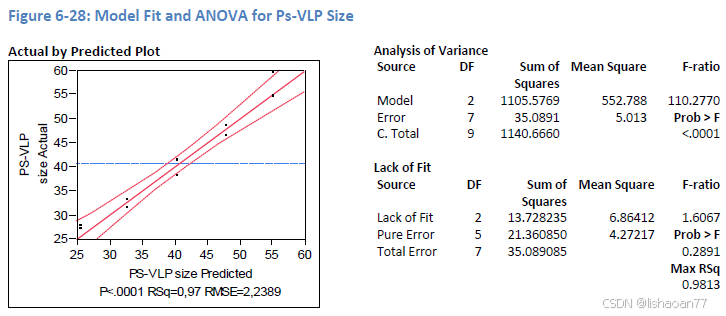
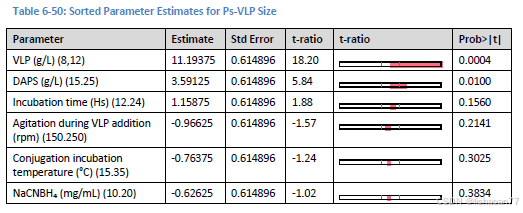
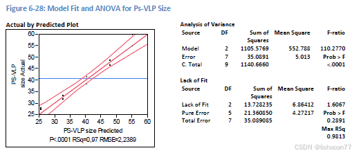
mod3 <- lm( y3 ~ (.), data = study6)
summary(mod3)
> summary(mod3)
Call:
lm.default(formula = y3 ~ (.), data = study6)
Residuals:
1 2 3 4 5 6 7 8 9 10
0.2095 0.3370 0.2095 0.2095 0.3370 0.3370 0.2095 0.6470 0.3370 -2.8330
Coefficients:
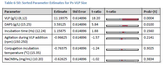
Estimate Std. Error t value Pr(>|t|)
(Intercept) 40.5630 0.5500 73.754 5.49e-06 ***
A 3.5913 0.6149 5.840 0.010002 *
B 11.1938 0.6149 18.204 0.000362 ***
C -0.7637 0.6149 -1.242 0.302458
D -0.9662 0.6149 -1.571 0.214127
E -0.6262 0.6149 -1.018 0.383437
F 1.1588 0.6149 1.884 0.156005
---
Signif. codes: 0 ‘***’ 0.001 ‘**’ 0.01 ‘*’ 0.05 ‘.’ 0.1 ‘ ’ 1
Residual standard error: 1.739 on 3 degrees of freedom
Multiple R-squared: 0.992, Adjusted R-squared: 0.9761
F-statistic: 62.35 on 6 and 3 DF, p-value: 0.003075
mod4 <- lm( y4 ~ (.), data = study6)
summary(mod4)
> summary(mod4)
Call:
lm.default(formula = y4 ~ (.), data = study6)
Residuals:
1 2 3 4 5 6 7 8 9 10
-2.05 0.45 -2.05 -2.05 0.45 0.45 -2.05 -1.30 0.45 7.70
Coefficients:
Estimate Std. Error t value Pr(>|t|)
(Intercept) 4.830e+01 1.619e+00 29.840 8.27e-05 ***
A -1.000e+00 1.810e+00 -0.553 0.6191
B -2.250e+00 1.810e+00 -1.243 0.3021
C 7.750e+00 1.810e+00 4.282 0.0234 *
D 2.500e+00 1.810e+00 1.381 0.2610
E 2.728e-15 1.810e+00 0.000 1.0000
F -2.500e-01 1.810e+00 -0.138 0.8989
---
Signif. codes: 0 ‘***’ 0.001 ‘**’ 0.01 ‘*’ 0.05 ‘.’ 0.1 ‘ ’ 1
Residual standard error: 5.119 on 3 degrees of freedom
Multiple R-squared: 0.8806, Adjusted R-squared: 0.6417
- statistic: 3.686 on 6 and 3 DF, p-value: 0.1558