当前位置：首页 > news >正文

DAY 44 预训练模型

news 来源：原创 2025/6/8 13:09:35

知识点回顾：

预训练的概念
常见的分类预训练模型
图像预训练模型的发展史
预训练的策略
预训练代码实战：resnet18

（一）预训练的概念

我们发现准确率最开始随着epoch的增加而增加。随着循环的更新，参数在不断发生更新。

所以参数的初始值对训练结果有很大的影响：

1. 如果最开始的初始值比较好，后续训练轮数就会少很多

2. 很有可能陷入局部最优值，不同的初始值可能导致陷入不同的局部最优值

所以很自然的想到，如果最开始能有比较好的参数，即可能导致未来训练次数少，也可能导致未来训练避免陷入局部最优解的问题。这就引入了一个概念，即预训练模型。如果别人在某些和我们目标数据类似的大规模数据集上做过训练，我们可以用他的训练参数来初始化我们的模型，这样我们的模型就比较容易收敛。

我们把用预训练模型的参数，然后接着在自己数据集上训练来调整该参数的过程叫做微调，这种思想叫做迁移学习。把预训练的过程叫做上游任务，把微调的过程叫做下游任务。

（二）常见的分类预训练模型

CNN架构预训练模型

模型	预训练数据集	核心特点	在CIFAR10上的适配要点
AlexNet	ImageNet	首次引入ReLU/局部响应归一化，参数量6000万+	需修改首层卷积核大小（原11x11→适配32x32）
VGG16	ImageNet	纯卷积堆叠，结构统一，参数量1.38亿	冻结前10层卷积，仅微调全连接层
ResNet18	ImageNet	残差连接解决梯度消失，参数量1100万	直接适配32x32输入，需调整池化层步长
MobileNetV2	ImageNet	深度可分离卷积，参数量350万+	轻量级设计，适合计算资源有限的场景

Transformer类预训练模型

模型	预训练数据集	核心特点	在CIFAR10上的适配要点
ViT-Base	ImageNet-21K	纯Transformer架构，参数量8600万	图像Resize至224x224，Patch大小设为4x4
Swin Transformer	ImageNet-22K	分层窗口注意力，参数量8000万+	需调整窗口大小适配小图像
DeiT	ImageNet	结合CNN归纳偏置，参数量2200万	轻量级Transformer，适合中小尺寸图像

适用于较大尺图像（如224x224），在CIFAR10上需上采样图像尺寸或调整Patch大小。

自监督预训练模型

模型	预训练方式	典型数据集	在CIFAR10上的优势
MoCo v3	对比学习	ImageNet	无需标签即可迁移，适合无标注数据
BEiT	掩码图像建模	ImageNet-22K	特征语义丰富，微调时收敛更快

无需人工标注，通过 pretext task（如掩码图像重建）学习特征，适合数据稀缺场景。

（三）图像预训练模型的发展史

模型	年份	提出团队	关键创新点	层数	参数量	ImageNet Top-5错误率	典型应用场景	预训练权重可用性
LeNet-5	1998	Yann LeCun等	首个CNN架构，卷积层+池化层+全连接层，Sigmoid激活函数	7	~60K	N/A	手写数字识别（MNIST）	无（历史模型）
AlexNet	2012	Alex Krizhevsky等	ReLU激活函数、Dropout、数据增强、GPU训练	8	60M	15.3%	大规模图像分类	PyTorch/TensorFlow官方支持
VGGNet	2014	Oxford VGG团队	统一3×3卷积核、多尺度特征提取、结构简洁	16/19	138M/144M	7.3%/7.0%	图像分类、目标检测基础骨干网络	PyTorch/TensorFlow官方支持
GoogLeNet	2014	Google	Inception模块（多分支并行卷积）、1×1卷积降维、全局平均池化	22	5M	6.7%	大规模图像分类	PyTorch/TensorFlow官方支持
ResNet	2015	何恺明等	残差连接（解决梯度消失）、Batch Normalization	18/50/152	11M/25M/60M	3.57%/3.63%/3.58%	图像/视频分类、检测、分割	PyTorch/TensorFlow官方支持
DenseNet	2017	Gao Huang等	密集连接（每层与后续所有层相连）、特征复用、参数效率高	121/169	8M/14M	2.80%	小数据集、医学图像处理	PyTorch/TensorFlow官方支持
MobileNet	2017	Google	深度可分离卷积（减少75%计算量）、轻量级设计	28	4.2M	7.4%	移动端图像分类/检测	PyTorch/TensorFlow官方支持
EfficientNet	2019	Google	复合缩放（同时优化深度、宽度、分辨率）、NAS搜索最佳配置	B0-B7	5.3M-66M	2.6% (B7)	高精度图像分类（资源受限场景）	PyTorch/TensorFlow官方支持

上图的层数，代表该模型不同的版本resnet有resnet18、resnet50、resnet152；efficientnet有efficientnet-b0、efficientnet-b1、efficientnet-b2、efficientnet-b3、efficientnet-b4等

其中ImageNet Top - 5 准确率是图像分类任务里的一种评估指标，用于衡量模型在 ImageNet 数据集上的分类性能，模型对图像进行分类预测，输出所有类别（共 1000 类）的概率，取概率排名前五的类别，只要这五个类别里包含人工标注的正确类别，就算预测正确。

总结：CNN 架构发展脉络

1. 早期探索（1990s-2010s）：LeNet 验证 CNN 可行性，但受限于计算和数据。

2. 深度学习复兴（2012-2015）：AlexNet、VGGNet、GoogLeNet 通过加深网络和结构创新突破性能。

3. 超深网络时代（2015 年后）：ResNet 解决退化问题，开启残差连接范式，后续模型围绕效率（MobileNet）、特征复用（DenseNet）、多分支结构（Inception）等方向优化。

（四）预训练的策略

需要找到预训练的模型结构并且加载模型参数

注意点：

1. 需要调用预训练模型和加载权重

2. 需要resize 图片让其可以适配模型

3. 需要修改最后的全连接层以适应数据集

其中，训练过程中，为了不破坏最开始的特征提取器的参数，最开始往往先冻结住特征提取器的参数，然后训练全连接层，大约在5-10个epoch后解冻训练。

主要做特征提取的部分叫做backbone骨干网络；负责融合提取的特征的部分叫做Featue Pyramid Network（FPN）；负责输出的预测部分的叫做Head。

import torch
import torch.nn as nn
import torch.optim as optim
from torchvision import datasets, transforms
from torch.utils.data import DataLoader
import matplotlib.pyplot as plt# 设置中文字体支持
plt.rcParams["font.family"] = ["SimHei"]
plt.rcParams['axes.unicode_minus'] = False  # 解决负号显示问题# 检查GPU是否可用
device = torch.device("cuda" if torch.cuda.is_available() else "cpu")
print(f"使用设备: {device}")# 1. 数据预处理（训练集增强，测试集标准化）
train_transform = transforms.Compose([transforms.RandomCrop(32, padding=4),transforms.RandomHorizontalFlip(),transforms.ColorJitter(brightness=0.2, contrast=0.2, saturation=0.2, hue=0.1),transforms.RandomRotation(15),transforms.ToTensor(),transforms.Normalize((0.4914, 0.4822, 0.4465), (0.2023, 0.1994, 0.2010))
])test_transform = transforms.Compose([transforms.ToTensor(),transforms.Normalize((0.4914, 0.4822, 0.4465), (0.2023, 0.1994, 0.2010))
])# 2. 加载CIFAR-10数据集
train_dataset = datasets.CIFAR10(root='./data',train=True,download=True,transform=train_transform
)test_dataset = datasets.CIFAR10(root='./data',train=False,transform=test_transform
)# 3. 创建数据加载器（可调整batch_size）
batch_size = 64
train_loader = DataLoader(train_dataset, batch_size=batch_size, shuffle=True)
test_loader = DataLoader(test_dataset, batch_size=batch_size, shuffle=False)# 4. 训练函数（支持学习率调度器）
def train(model, train_loader, test_loader, criterion, optimizer, scheduler, device, epochs):model.train()  # 设置为训练模式train_loss_history = []test_loss_history = []train_acc_history = []test_acc_history = []all_iter_losses = []iter_indices = []for epoch in range(epochs):running_loss = 0.0correct_train = 0total_train = 0for batch_idx, (data, target) in enumerate(train_loader):data, target = data.to(device), target.to(device)optimizer.zero_grad()output = model(data)loss = criterion(output, target)loss.backward()optimizer.step()# 记录Iteration损失iter_loss = loss.item()all_iter_losses.append(iter_loss)iter_indices.append(epoch * len(train_loader) + batch_idx + 1)# 统计训练指标running_loss += iter_loss_, predicted = output.max(1)total_train += target.size(0)correct_train += predicted.eq(target).sum().item()# 每100批次打印进度if (batch_idx + 1) % 100 == 0:print(f"Epoch {epoch+1}/{epochs} | Batch {batch_idx+1}/{len(train_loader)} "f"| 单Batch损失: {iter_loss:.4f}")# 计算 epoch 级指标epoch_train_loss = running_loss / len(train_loader)epoch_train_acc = 100. * correct_train / total_train# 测试阶段model.eval()correct_test = 0total_test = 0test_loss = 0.0with torch.no_grad():for data, target in test_loader:data, target = data.to(device), target.to(device)output = model(data)test_loss += criterion(output, target).item()_, predicted = output.max(1)total_test += target.size(0)correct_test += predicted.eq(target).sum().item()epoch_test_loss = test_loss / len(test_loader)epoch_test_acc = 100. * correct_test / total_test# 记录历史数据train_loss_history.append(epoch_train_loss)test_loss_history.append(epoch_test_loss)train_acc_history.append(epoch_train_acc)test_acc_history.append(epoch_test_acc)# 更新学习率调度器if scheduler is not None:scheduler.step(epoch_test_loss)# 打印 epoch 结果print(f"Epoch {epoch+1} 完成 | 训练损失: {epoch_train_loss:.4f} "f"| 训练准确率: {epoch_train_acc:.2f}% | 测试准确率: {epoch_test_acc:.2f}%")# 绘制损失和准确率曲线plot_iter_losses(all_iter_losses, iter_indices)plot_epoch_metrics(train_acc_history, test_acc_history, train_loss_history, test_loss_history)return epoch_test_acc  # 返回最终测试准确率# 5. 绘制Iteration损失曲线
def plot_iter_losses(losses, indices):plt.figure(figsize=(10, 4))plt.plot(indices, losses, 'b-', alpha=0.7)plt.xlabel('Iteration（Batch序号）')plt.ylabel('损失值')plt.title('训练过程中的Iteration损失变化')plt.grid(True)plt.show()# 6. 绘制Epoch级指标曲线
def plot_epoch_metrics(train_acc, test_acc, train_loss, test_loss):epochs = range(1, len(train_acc) + 1)plt.figure(figsize=(12, 5))# 准确率曲线plt.subplot(1, 2, 1)plt.plot(epochs, train_acc, 'b-', label='训练准确率')plt.plot(epochs, test_acc, 'r-', label='测试准确率')plt.xlabel('Epoch')plt.ylabel('准确率 (%)')plt.title('准确率随Epoch变化')plt.legend()plt.grid(True)# 损失曲线plt.subplot(1, 2, 2)plt.plot(epochs, train_loss, 'b-', label='训练损失')plt.plot(epochs, test_loss, 'r-', label='测试损失')plt.xlabel('Epoch')plt.ylabel('损失值')plt.title('损失值随Epoch变化')plt.legend()plt.grid(True)plt.tight_layout()plt.show()
# 导入ResNet模型
from torchvision.models import resnet18# 定义ResNet18模型（支持预训练权重加载）
def create_resnet18(pretrained=True, num_classes=10):# 加载预训练模型（ImageNet权重）model = resnet18(pretrained=pretrained)# 修改最后一层全连接层，适配CIFAR-10的10分类任务in_features = model.fc.in_featuresmodel.fc = nn.Linear(in_features, num_classes)# 将模型转移到指定设备（CPU/GPU）model = model.to(device)return model
# 创建ResNet18模型（加载ImageNet预训练权重，不进行微调）
model = create_resnet18(pretrained=True, num_classes=10)
model.eval()  # 设置为推理模式# 测试单张图片（示例）
from torchvision import utils# 从测试数据集中获取一张图片
dataiter = iter(test_loader)
images, labels = dataiter.next()
images = images[:1].to(device)  # 取第1张图片# 前向传播
with torch.no_grad():outputs = model(images)_, predicted = torch.max(outputs.data, 1)# 显示图片和预测结果
plt.imshow(utils.make_grid(images.cpu(), normalize=True).permute(1, 2, 0))
plt.title(f"预测类别: {predicted.item()}")
plt.axis('off')
plt.show()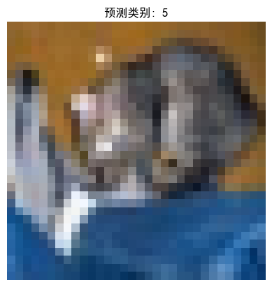

import torch
import torch.nn as nn
import torch.optim as optim
from torchvision import datasets, transforms, models
from torch.utils.data import DataLoader
import matplotlib.pyplot as plt
import os# 设置中文字体支持
plt.rcParams["font.family"] = ["SimHei"]
plt.rcParams['axes.unicode_minus'] = False  # 解决负号显示问题# 检查GPU是否可用
device = torch.device("cuda" if torch.cuda.is_available() else "cpu")
print(f"使用设备: {device}")# 1. 数据预处理（训练集增强，测试集标准化）
train_transform = transforms.Compose([transforms.RandomCrop(32, padding=4),transforms.RandomHorizontalFlip(),transforms.ColorJitter(brightness=0.2, contrast=0.2, saturation=0.2, hue=0.1),transforms.RandomRotation(15),transforms.ToTensor(),transforms.Normalize((0.4914, 0.4822, 0.4465), (0.2023, 0.1994, 0.2010))
])test_transform = transforms.Compose([transforms.ToTensor(),transforms.Normalize((0.4914, 0.4822, 0.4465), (0.2023, 0.1994, 0.2010))
])# 2. 加载CIFAR-10数据集
train_dataset = datasets.CIFAR10(root='./data',train=True,download=True,transform=train_transform
)test_dataset = datasets.CIFAR10(root='./data',train=False,transform=test_transform
)# 3. 创建数据加载器
batch_size = 64
train_loader = DataLoader(train_dataset, batch_size=batch_size, shuffle=True)
test_loader = DataLoader(test_dataset, batch_size=batch_size, shuffle=False)# 4. 定义ResNet18模型
def create_resnet18(pretrained=True, num_classes=10):model = models.resnet18(pretrained=pretrained)# 修改最后一层全连接层in_features = model.fc.in_featuresmodel.fc = nn.Linear(in_features, num_classes)return model.to(device)# 5. 冻结/解冻模型层的函数
def freeze_model(model, freeze=True):"""冻结或解冻模型的卷积层参数"""# 冻结/解冻除fc层外的所有参数for name, param in model.named_parameters():if 'fc' not in name:param.requires_grad = not freeze# 打印冻结状态frozen_params = sum(p.numel() for p in model.parameters() if not p.requires_grad)total_params = sum(p.numel() for p in model.parameters())if freeze:print(f"已冻结模型卷积层参数 ({frozen_params}/{total_params} 参数)")else:print(f"已解冻模型所有参数 ({total_params}/{total_params} 参数可训练)")return model# 6. 训练函数（支持阶段式训练）
def train_with_freeze_schedule(model, train_loader, test_loader, criterion, optimizer, scheduler, device, epochs, freeze_epochs=5):"""前freeze_epochs轮冻结卷积层，之后解冻所有层进行训练"""train_loss_history = []test_loss_history = []train_acc_history = []test_acc_history = []all_iter_losses = []iter_indices = []# 初始冻结卷积层if freeze_epochs > 0:model = freeze_model(model, freeze=True)for epoch in range(epochs):# 解冻控制：在指定轮次后解冻所有层if epoch == freeze_epochs:model = freeze_model(model, freeze=False)# 解冻后调整优化器（可选）optimizer.param_groups[0]['lr'] = 1e-4  # 降低学习率防止过拟合model.train()  # 设置为训练模式running_loss = 0.0correct_train = 0total_train = 0for batch_idx, (data, target) in enumerate(train_loader):data, target = data.to(device), target.to(device)optimizer.zero_grad()output = model(data)loss = criterion(output, target)loss.backward()optimizer.step()# 记录Iteration损失iter_loss = loss.item()all_iter_losses.append(iter_loss)iter_indices.append(epoch * len(train_loader) + batch_idx + 1)# 统计训练指标running_loss += iter_loss_, predicted = output.max(1)total_train += target.size(0)correct_train += predicted.eq(target).sum().item()# 每100批次打印进度if (batch_idx + 1) % 100 == 0:print(f"Epoch {epoch+1}/{epochs} | Batch {batch_idx+1}/{len(train_loader)} "f"| 单Batch损失: {iter_loss:.4f}")# 计算 epoch 级指标epoch_train_loss = running_loss / len(train_loader)epoch_train_acc = 100. * correct_train / total_train# 测试阶段model.eval()correct_test = 0total_test = 0test_loss = 0.0with torch.no_grad():for data, target in test_loader:data, target = data.to(device), target.to(device)output = model(data)test_loss += criterion(output, target).item()_, predicted = output.max(1)total_test += target.size(0)correct_test += predicted.eq(target).sum().item()epoch_test_loss = test_loss / len(test_loader)epoch_test_acc = 100. * correct_test / total_test# 记录历史数据train_loss_history.append(epoch_train_loss)test_loss_history.append(epoch_test_loss)train_acc_history.append(epoch_train_acc)test_acc_history.append(epoch_test_acc)# 更新学习率调度器if scheduler is not None:scheduler.step(epoch_test_loss)# 打印 epoch 结果print(f"Epoch {epoch+1} 完成 | 训练损失: {epoch_train_loss:.4f} "f"| 训练准确率: {epoch_train_acc:.2f}% | 测试准确率: {epoch_test_acc:.2f}%")# 绘制损失和准确率曲线plot_iter_losses(all_iter_losses, iter_indices)plot_epoch_metrics(train_acc_history, test_acc_history, train_loss_history, test_loss_history)return epoch_test_acc  # 返回最终测试准确率# 7. 绘制Iteration损失曲线
def plot_iter_losses(losses, indices):plt.figure(figsize=(10, 4))plt.plot(indices, losses, 'b-', alpha=0.7)plt.xlabel('Iteration（Batch序号）')plt.ylabel('损失值')plt.title('训练过程中的Iteration损失变化')plt.grid(True)plt.show()# 8. 绘制Epoch级指标曲线
def plot_epoch_metrics(train_acc, test_acc, train_loss, test_loss):epochs = range(1, len(train_acc) + 1)plt.figure(figsize=(12, 5))# 准确率曲线plt.subplot(1, 2, 1)plt.plot(epochs, train_acc, 'b-', label='训练准确率')plt.plot(epochs, test_acc, 'r-', label='测试准确率')plt.xlabel('Epoch')plt.ylabel('准确率 (%)')plt.title('准确率随Epoch变化')plt.legend()plt.grid(True)# 损失曲线plt.subplot(1, 2, 2)plt.plot(epochs, train_loss, 'b-', label='训练损失')plt.plot(epochs, test_loss, 'r-', label='测试损失')plt.xlabel('Epoch')plt.ylabel('损失值')plt.title('损失值随Epoch变化')plt.legend()plt.grid(True)plt.tight_layout()plt.show()# 主函数：训练模型
def main():# 参数设置epochs = 10  # 总训练轮次freeze_epochs = 5  # 冻结卷积层的轮次learning_rate = 1e-3  # 初始学习率weight_decay = 1e-4  # 权重衰减# 创建ResNet18模型（加载预训练权重）model = create_resnet18(pretrained=True, num_classes=10)# 定义优化器和损失函数optimizer = optim.Adam(model.parameters(), lr=learning_rate, weight_decay=weight_decay)criterion = nn.CrossEntropyLoss()# 定义学习率调度器scheduler = optim.lr_scheduler.ReduceLROnPlateau(optimizer, mode='min', factor=0.5, patience=2, verbose=True)# 开始训练（前5轮冻结卷积层，之后解冻）final_accuracy = train_with_freeze_schedule(model=model,train_loader=train_loader,test_loader=test_loader,criterion=criterion,optimizer=optimizer,scheduler=scheduler,device=device,epochs=epochs,freeze_epochs=freeze_epochs)print(f"训练完成！最终测试准确率: {final_accuracy:.2f}%")# # 保存模型# torch.save(model.state_dict(), 'resnet18_cifar10_finetuned.pth')# print("模型已保存至: resnet18_cifar10_finetuned.pth")if __name__ == "__main__":main()

使用设备: cpu
Files already downloaded and verified
已冻结模型卷积层参数 (11176512/11181642 参数)
Epoch 1/10 | Batch 100/782 | 单Batch损失: 2.1392
Epoch 1/10 | Batch 200/782 | 单Batch损失: 1.9631
Epoch 1/10 | Batch 300/782 | 单Batch损失: 2.1302
Epoch 1/10 | Batch 400/782 | 单Batch损失: 1.9457
Epoch 1/10 | Batch 500/782 | 单Batch损失: 1.8974
Epoch 1/10 | Batch 600/782 | 单Batch损失: 1.7904
Epoch 1/10 | Batch 700/782 | 单Batch损失: 1.6946
Epoch 1 完成 | 训练损失: 1.9604 | 训练准确率: 30.52% | 测试准确率: 32.52%
Epoch 2/10 | Batch 100/782 | 单Batch损失: 1.6137
Epoch 2/10 | Batch 200/782 | 单Batch损失: 1.8684
Epoch 2/10 | Batch 300/782 | 单Batch损失: 1.8782
Epoch 2/10 | Batch 400/782 | 单Batch损失: 1.8397
Epoch 2/10 | Batch 500/782 | 单Batch损失: 1.8395
Epoch 2/10 | Batch 600/782 | 单Batch损失: 1.9212
Epoch 2/10 | Batch 700/782 | 单Batch损失: 1.9270
Epoch 2 完成 | 训练损失: 1.8652 | 训练准确率: 33.66% | 测试准确率: 35.49%
Epoch 3/10 | Batch 100/782 | 单Batch损失: 1.7297
Epoch 3/10 | Batch 200/782 | 单Batch损失: 1.7276
Epoch 3/10 | Batch 300/782 | 单Batch损失: 1.9344
Epoch 3/10 | Batch 400/782 | 单Batch损失: 1.5545
Epoch 3/10 | Batch 500/782 | 单Batch损失: 1.6845
Epoch 3/10 | Batch 600/782 | 单Batch损失: 1.8561
Epoch 3/10 | Batch 700/782 | 单Batch损失: 1.8792
Epoch 3 完成 | 训练损失: 1.8562 | 训练准确率: 34.27% | 测试准确率: 33.67%
Epoch 4/10 | Batch 100/782 | 单Batch损失: 1.8853
Epoch 4/10 | Batch 200/782 | 单Batch损失: 1.9597
Epoch 4/10 | Batch 300/782 | 单Batch损失: 1.9182
Epoch 4/10 | Batch 400/782 | 单Batch损失: 1.8609
Epoch 4/10 | Batch 500/782 | 单Batch损失: 1.8729
Epoch 4/10 | Batch 600/782 | 单Batch损失: 1.8401
Epoch 4/10 | Batch 700/782 | 单Batch损失: 1.9293
Epoch 4 完成 | 训练损失: 1.8592 | 训练准确率: 34.06% | 测试准确率: 34.32%
Epoch 5/10 | Batch 100/782 | 单Batch损失: 1.9967
Epoch 5/10 | Batch 200/782 | 单Batch损失: 2.0677
Epoch 5/10 | Batch 300/782 | 单Batch损失: 1.7265
Epoch 5/10 | Batch 400/782 | 单Batch损失: 1.8522
Epoch 5/10 | Batch 500/782 | 单Batch损失: 1.6979
Epoch 5/10 | Batch 600/782 | 单Batch损失: 1.8386
Epoch 5/10 | Batch 700/782 | 单Batch损失: 1.6844
Epoch 5 完成 | 训练损失: 1.8464 | 训练准确率: 34.40% | 测试准确率: 34.69%
已解冻模型所有参数 (11181642/11181642 参数可训练)
Epoch 6/10 | Batch 100/782 | 单Batch损失: 1.6713
Epoch 6/10 | Batch 200/782 | 单Batch损失: 1.2268
Epoch 6/10 | Batch 300/782 | 单Batch损失: 1.4253
Epoch 6/10 | Batch 400/782 | 单Batch损失: 1.4628
Epoch 6/10 | Batch 500/782 | 单Batch损失: 1.0016
Epoch 6/10 | Batch 600/782 | 单Batch损失: 1.2681
Epoch 6/10 | Batch 700/782 | 单Batch损失: 1.2972
Epoch 6 完成 | 训练损失: 1.3021 | 训练准确率: 54.32% | 测试准确率: 69.41%
Epoch 7/10 | Batch 100/782 | 单Batch损失: 0.9048
Epoch 7/10 | Batch 200/782 | 单Batch损失: 1.0555
Epoch 7/10 | Batch 300/782 | 单Batch损失: 0.8342
Epoch 7/10 | Batch 400/782 | 单Batch损失: 1.0666
Epoch 7/10 | Batch 500/782 | 单Batch损失: 1.0574
Epoch 7/10 | Batch 600/782 | 单Batch损失: 0.9818
Epoch 7/10 | Batch 700/782 | 单Batch损失: 0.9298
Epoch 7 完成 | 训练损失: 0.9814 | 训练准确率: 65.86% | 测试准确率: 74.15%
Epoch 8/10 | Batch 100/782 | 单Batch损失: 0.8358
Epoch 8/10 | Batch 200/782 | 单Batch损失: 1.0294
Epoch 8/10 | Batch 300/782 | 单Batch损失: 1.0704
Epoch 8/10 | Batch 400/782 | 单Batch损失: 0.7411
Epoch 8/10 | Batch 500/782 | 单Batch损失: 0.7433
Epoch 8/10 | Batch 600/782 | 单Batch损失: 0.7691
Epoch 8/10 | Batch 700/782 | 单Batch损失: 0.9913
Epoch 8 完成 | 训练损失: 0.8669 | 训练准确率: 69.76% | 测试准确率: 76.80%
Epoch 9/10 | Batch 100/782 | 单Batch损失: 0.9027
Epoch 9/10 | Batch 200/782 | 单Batch损失: 0.9157
Epoch 9/10 | Batch 300/782 | 单Batch损失: 0.6013
Epoch 9/10 | Batch 400/782 | 单Batch损失: 0.7628
Epoch 9/10 | Batch 500/782 | 单Batch损失: 0.7645
Epoch 9/10 | Batch 600/782 | 单Batch损失: 0.8824
Epoch 9/10 | Batch 700/782 | 单Batch损失: 0.6547
Epoch 9 完成 | 训练损失: 0.7983 | 训练准确率: 72.32% | 测试准确率: 78.79%
Epoch 10/10 | Batch 100/782 | 单Batch损失: 0.7249
Epoch 10/10 | Batch 200/782 | 单Batch损失: 0.5305
Epoch 10/10 | Batch 300/782 | 单Batch损失: 1.0288
Epoch 10/10 | Batch 400/782 | 单Batch损失: 0.6281
Epoch 10/10 | Batch 500/782 | 单Batch损失: 1.0929
Epoch 10/10 | Batch 600/782 | 单Batch损失: 0.8086
Epoch 10/10 | Batch 700/782 | 单Batch损失: 0.8518
Epoch 10 完成 | 训练损失: 0.7469 | 训练准确率: 74.02% | 测试准确率: 79.85%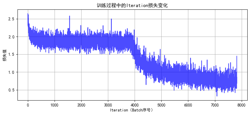

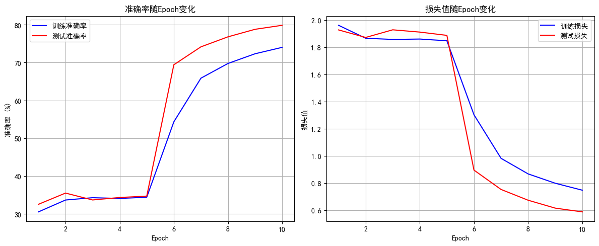
明显现象：

1. 解冻后几个epoch即可达到之前cnn训练20轮的效果，这是预训练的优势

2. 由于训练集用了 RandomCrop（随机裁剪）、RandomHorizontalFlip（随机水平翻转）、ColorJitter（颜色抖动）等数据增强操作，这会让训练时模型看到的图片有更多 “干扰” 或变形。比如一张汽车图片，训练时可能被裁剪成只显示局部、颜色也有变化，模型学习难度更高；而测试集是标准的、没增强的图片，模型预测相对轻松，就可能出现训练集准确率暂时低于测试集的情况，尤其在训练前期增强对模型影响更明显。随着训练推进，模型适应增强后会缓解。

3. 最后收敛后的效果超过非预训练模型的80%,大幅提升

#介绍残差：

残差连接的核心思想是：